srukf

Run one update of a square-root unscented (sigma point) Kalman filter. The advantage of a "square-root" UKF over a traditional UKF is that the covariance can be maintained in a more numerically stable way.

[x_k, S_k] = srukf( ...
    t_km1, t_k, x_km1, S_km1, u_km1, z_k, ...
    f, h, sqQ_km1, sqR_k, ...
    alpha, beta, kappa, ...
    (etc.))

Inputs

t_km1	Time at sample k-1
t_k	Time at sample k
x_km1	State estimate at sample k-1
S_km1	Cholesky factor (lower diagonal) of the estimate covariance at sample k-1, such that the covariance is `S_km1 * S_km1.'`.
u_km1	Input vector at sample k-1
z_k	Measurement at sample k
f	Propagation function with interface: `x_k = f(t_km1, t_k, x_km1, u_km1, q_km1)` where `q_km1` is the process noise at sample k-1
h	Measurement function with interface: `z_k = h(t_k, x_k, u_km1, r_k)` where `r_k` is the measurement noise at sample k
sqQ	Matrix square root of the pocess noise covariance at k-1
sqR	Matrix square root of the measurement noise covariance at k
alpha	Optional tuning parameter, often 0.001
beta	Optional tuning parameter, with 2 being optimal for Gaussian estimation error
kappa	Optional tuning parameter, often 3 - `nx`, where `nx` is the dimension of the state
(etc.)	Additional arguments to be passed to f and h after their normal arguments

Outputs

x	Upated estimate at sample k
S	Updated Cholesky factor of the estimate covariance at k

Example

We can quickly create a simulation for discrete, dynamic system, generate noisy measurements of the system over time, and pass these to a square-root unscented Kalman filter.

First, define the discrete system.

rng(1);
dt    = 0.1;                                  % Time step
F_km1 = expm([0 1; -1 0]*dt);                 % State transition matrix
H_k   = [1 0];                                % Observation matrix
G_km1 = [0.5*dt^2; dt];                       % Process-noise-to-state map
Q_km1 = G_km1 * 0.5^2 * G_km1.';              % Process noise variance
R_k   = 0.1;                                  % Meas. noise covariance

The srukf algorithm uses the sqrts of the process and measurement noise as well. These can be a cholesky factor or the form returned by sqrtpsdm; it doesn't matter.

sqQ = sqrtpsdm(Q_km1);
sqR = sqrtpsdm(R_k);

Make propagation and observation functions. These are just linear for this example, but srukf is meant for nonlinear functions.

f = @(t_km1, t_k, x_km1, u_km1, q_km1) F_km1 * x_km1 + q_km1;
h = @(t_k, x_k, u_km1, r_k) H_k * x_k + r_k;

Now, we'll define the simulation's time step and initial conditions. Note that we define the initial estimate and set the truth as a small error from the estimate (using the covariance).

n       = 100;                     % Number of samples to simulate
x_hat_0 = [1; 0];                  % Initial estimate
P       = diag([0.5 1].^2);        % Initial estimate covariance
S       = sqrtpsdm(P, 'L');        % Initial sqrt of the covariance
x_0     = x_hat_0 + mnddraw(P, 1); % Initial true state

Now we'll just write a loop for the discrete simulation.

% Storage for time histories
x     = [x_0, zeros(2, n-1)];                         % True state
x_hat = [x_hat_0, zeros(2, n-1)];                     % Estimate
z     = [H_k * x_0 + mnddraw(R_k, 1), zeros(1, n-1)]; % Measurement
 
% Simulate each sample over time.
for k = 2:n
 
    % Propagate the true state.
    x(:, k) = F_km1 * x(:, k-1) + mnddraw(Q_km1, 1);
    
    % Create the real measurement at sample k.
    z(:, k) = H_k * x(:, k) + mnddraw(R_k, 1);
 
    % Run the Kalman correction.
    [x_hat(:,k), S] = srukf((k-1)*dt, k*dt, x_hat(:,k-1), S, [], z(:,k),...
                            f, h, sqQ, sqR);
 
end

Plot the results.

figure(1);
clf();
t = 0:dt:(n-1)*dt;
plot(t, x, ...
     t, z, '.', ...
     t, x_hat, '--');
legend('True x1', 'True x2', 'Meas.', 'Est. x1', 'Est. x2');
xlabel('Time');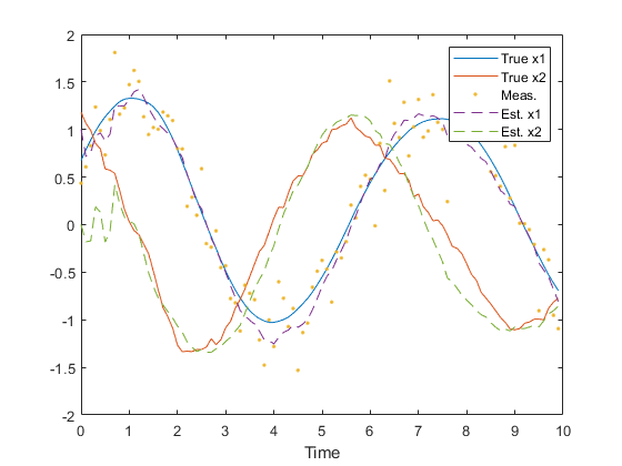

Note how similar this example is to the example of ukf.

Reference

Wan, Eric A. and Rudoph van der Merwe. "The Unscented Kalman Filter." Kalman Filtering and Neural Networks. Ed. Simon Haykin. New York: John Wiley & Sons, Inc., 2001. Print. Pages 273-275.

Docs

srukf

Inputs

Outputs

Example

Reference

See Also

Table of Contents