kfc

Perform a Kalman correction of the prior state and covariance. This can be used for a linear Kalman filter or for an extended Kalman filter, as they share the same update process.

This is perhaps the most basic form of a Kalman correction for a Kalman filter, and utilizes the generic Joseph form of covariance update for numerical stability.

[x_k, P_k] = kfc(P_km1, y_k, F_km1, H_k, Q_km1, R_k)

Inputs

P_km1	State estimate covariance at sample k-1
y_k	Innovation vector (measurement - prediction) at sample k
F_km1	State transition matrix at sample k-1
H_k	Observation matrix at sample k
Q_km1	Process noise at sample k
R_k	Measurement noise at sample k

Outputs:

dx	State estimate correction for sample k
P_k	Updated state covariance for sample k

Example

We can quickly create a simulation for discrete, dynamic system, generate noisy measurements of the system over time, and make a Kalman filter, where here we propagate manually and then call kfc only for the Kalman correction.

First, define the discrete system.

rng(1);
dt    = 0.1;                                  % Time step
F_km1 = expm([0 1; -1 0]*dt);                 % State transition matrix
H_k   = [1 0];                                % Observation matrix
Q_km1 = 0.5^2 * [0.5*dt^2; dt]*[0.5*dt^2 dt]; % Process noise covariance
R_k   = 0.1;                                  % Meas. noise covariance

Now, we'll define the simulation's time step and initial conditions. Note that we define the initial estimate and set the truth as a small error from the estimate (using the covariance).

n       = 100;                     % Number of samples to simulate
x_hat_0 = [1; 0];                  % Initial estimate
P       = diag([0.5 1].^2);        % Initial estimate covariance
x_0     = x_hat_0 + mnddraw(P, 1); % Initial true state

Now we'll just write a loop for the discrete simulation.

% Storage for time histories
x     = [x_0, zeros(2, n-1)];                         % True state
x_hat = [x_hat_0, zeros(2, n-1)];                     % Estimate
z     = [H_k * x_0 + mnddraw(R_k, 1), zeros(1, n-1)]; % Measurement
 
% Simulate each sample over time.
for k = 2:n
 
    % Propagate the true state.
    x(:, k) = F_km1 * x(:, k-1) + mnddraw(Q_km1, 1);
    
    % Create the real measurement at sample k.
    z(:, k) = H_k * x(:, k) + mnddraw(R_k, 1);
 
    % Predict the state and observation.
    x_hat_kkm1 = F_km1 * x_hat(:, k-1);
    z_hat      = H_k * x_hat_kkm1;
 
    % Calculate the innovation.
    y_k = z(:, k) - z_hat;
 
    % Run the Kalman correction.
    [dx, P] = kfc(y_k, P, F_km1, H_k, Q_km1, R_k);
    x_hat(:, k) = x_hat_kkm1 + dx;
                       
end

Plot the results.

figure(1);
clf();
t = 0:dt:(n-1)*dt;
h = plot(t, x, ...
         t, z, '.', ...
         t, x_hat, '--');
legend('True x1', 'True x2', 'Meas.', 'Est. x1', 'Est. x2');
xlabel('Time');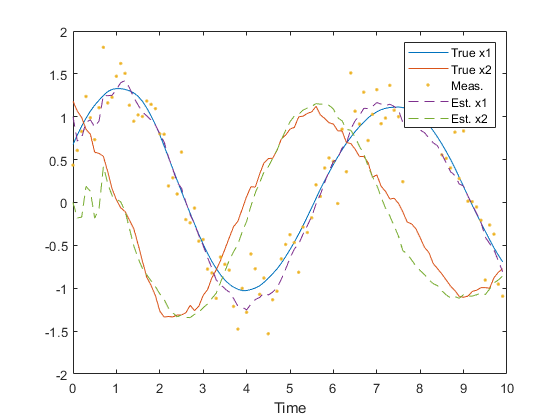

Docs

kfc

Inputs

Example

See Also

Table of Contents