by An Uncommon Lab

autocorrelate

Performs autocorrelation of data over n runs. x should be an nx-ns-nr matrix, where nx is the dimension of the state, ns is the number of samples, and nr is the number of runs. This function is used to test the "whiteness" of a multi-state signal recorded over multiple runs. It can provide various types of autocorrelation. If the number of runs is greater than 1, the correlations are normalized by default and assume the input is (intended to be) zero mean. If x is zero-mean and white, then the autocorrelation values between any different samples will be small (between the bounds returned in b), while the autocorrelation value of any sample with itself will be 1.

Type 1: Returns an nx-ns-ns matrix, xc, where xc(3, 5, 9) is the autocorrelation of the third state on sample 5 with that of sample 9, with the autocorrelation averaged across runs.

Type 2: Returns an nx-nL matrix, xc, where xc(3, 13) is the autocorrelation of all samples of the third state with a lag of 13-1 samples, again averaged across runs and normalized by the number of samples, where nL is the number of lags+1 (the +1 is to accomodate the autocorrelation of a sample with itself at position 1).

Type 3: Returns an nx-ns-nL matrix, xc, where xc(2, 5, 9) is the autocorrelation of the second state at sample 5 with a lag of 9-1 samples, again averaged across runs, where nL is as above.

xc         = autocorrelate(x)
xc         = autocorrelate(x, type)
[xc, f, b] = autocorrelate(x, type, p)
[xc, f, b] = autocorrelate(x, type, p, varargin)

Inputs

Outputs

Options

UseFullStateError When this option is specified, the components of the state are not treated separately, but rather the autocorrelation is considered on the entire state relation x(:, k, r).' * x(:, j, r) for some run, r, between samples k and j. When using this option, the first dimension of the output will be 1 instead of nx.

Normalize By default, the data is normalized at each sample by calculating the standard error (standard deviation assuming the samples are zero mean) and dividing this from the relevant states and samples. This causes the autocorrelation between the same states at the same samples to be unity.

NumLags By default, the autocorrelation is calculated for lags from 0 to the number of samples. If fewer are needed, this option can be used to specify the required number of lags.

Plot Set true to plot the results.

Example

Let's generate a vector of white noise and see that it passes the "whiteness" test (the appropriate amount of data is within the theoretical probability bounds) for the 3 types of autocorrelation.

nx = 2;    % 2 states
ns = 100;  % 100 samples per run
nr = 50;   % 50 runs
x  = 5 * randn(nx, ns, nr); % Gaussian data -- no real correlation

Type 1: Which samples correlate with which others?

figure(1);
[xc1, f1, b1] = autocorrelate(x, 1, 0.95, 'Plot', true);
size(xc1)

Percent of data in theoretical 95.0% bounds: 95.0%
ans =
     2   100   100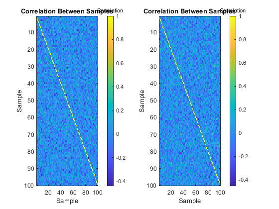

Type 2: What lags demonstrate correlation?

figure(2);
[xc2, f2, b2] = autocorrelate(x, 2, 0.95, 'Plot', true);
size(xc2)

Percent of data in theoretical 95.0% bounds: 97.5%
ans =
     2   100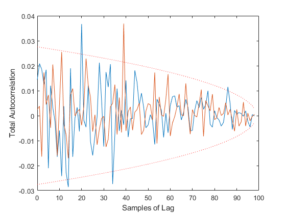

Type 3: Which elements of the state demonstrate autocorrelation over a small number of samples?

figure(3);
[xc3, f3, b3] = autocorrelate(x, 3, 0.95, 'NumLags', 5, 'Plot', true);
size(xc3)

Percent of data in theoretical 95.0% bounds: 94.9%
ans =
     2   100     6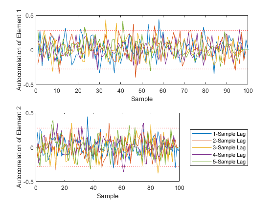

See Also

normerr, kffmct