by An Uncommon Lab

kffmct

Perform Monte-Carlo testing of a filter used in conjunction with kff. This makes Monte-Carlo testing very easy to do. It requires that the filter be set up using the kffoptions structure.

Interfaces

The simplest interface is:

[...] = kffmct(nr, ts, dt, x_hat_0, P_0, options);

where nr is the number of simulations to run, ts contains the state and stop times [t_start, t_stop], dt is the time step, x_hat_0 is the initial state estimate, and P_0 is the initial covariance.

The true initial state of each run will be randomly displaced from x_hat_0 by a Gaussian draw from P_0. The simulation will then propagate and create noisy measurements using the propagation and measurement functions from the options structure, along with the appropriate covariance matrices.

If the filter uses an input vector, one can provide a function, u_fcn, to create an input vector on each sample:

[...] = kffmct(nr, ts, dt, x_hat_0, P_0, u_fcn, options);

This function will be called on each time step to produce the input vector used for that step.

Consider covariance can be used too.

[...] = kffmct(nr, ts, dt, x_hat_0, P_0, P_xc_0, u_fcn, options);

where P_xc_0 is the initial covariance between the state and consider parameters.

Making the Monte-Carlo test more interesting is the ability to use different functions for the truth than for the filter. This allows one to use a more complex/realistic simulation than the filter uses to determine how well the filter will function in its real-world application. To do this, pass the true functions to kffmct.

[...] = kffmct(nr, ts, dt, x_hat_0, P_0, f, Q, h, R, options)

where f is the propagation function, Q is the process noise covariance matrix (or a function that returns the covariance matrix), h is the observation function, and R is the measurement noise covariance matrix (or function return such).

The truth can also include u_fcn:

[...] = kffmct(nr, ts, dt, x_hat_0, P_0, u_fcn, f, Q, h, R, options)

The different truth can also use different consider covariance.

[...] = kffmct(nr, ts, dt, x_hat_0, P_0, P_xc_0, u_fcn, ...
               f, F_c, Q, h, H_c, R, P_cc, options);

where F_c and H_c are the Jacobians of the propagation and observation functions wrt the consider parameters and P_cc is the consider covariance matrix.

All invocations output the same set of data:

[t, x, x_hat, P, P_xc, y, S, z_hat] = kffmct(...);

See the table below for the definition of these outputs.

Here is a summary of the interfaces (dropping subscripts for legibility):

kffmct(nr, ts, dt, xh0, P0, opt);
kffmct(nr, ts, dt, xh0, P0, ufcn, opt);
kffmct(nr, ts, dt, xh0, P0, Pxc0, ufcn, opt);
kffmct(nr, ts, dt, xh0, P0, f, Q, h, R, opt);
kffmct(nr, ts, dt, xh0, P0, ufcn, f, Q, h, R, opt);
kffmct(nr, ts, dt, xh0, P0, Pxc0, ufcn, f, Q, h, R, opt);
kffmct(nr, ts, dt, xh0, P0, Pxc0, ufcn, f, Q, h, R, Pc, opt);
kffmct(nr, ts, dt, xh0, P0, Pxc0, f, Fc, Q, h, Hc, R, Pc, opt);
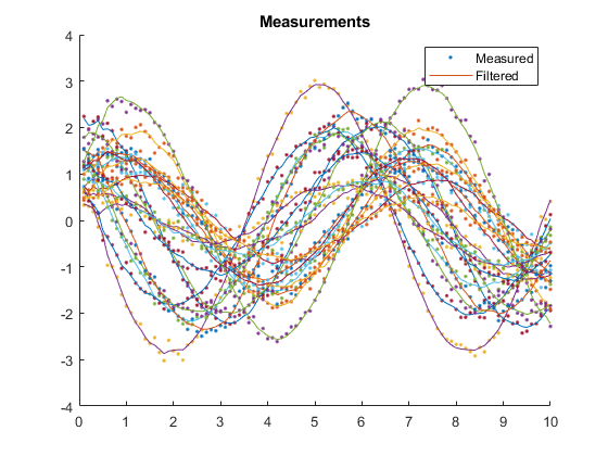
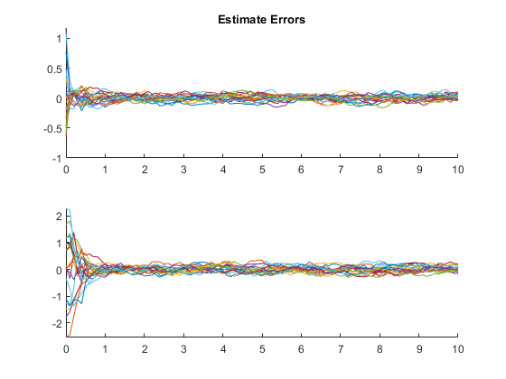
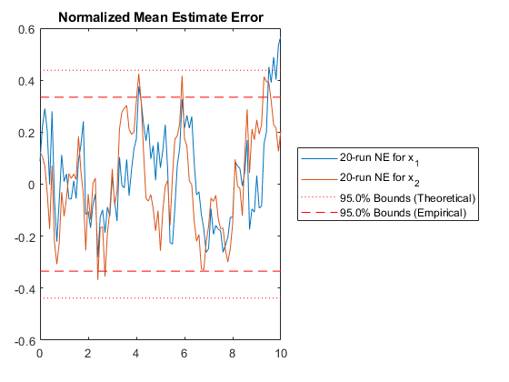
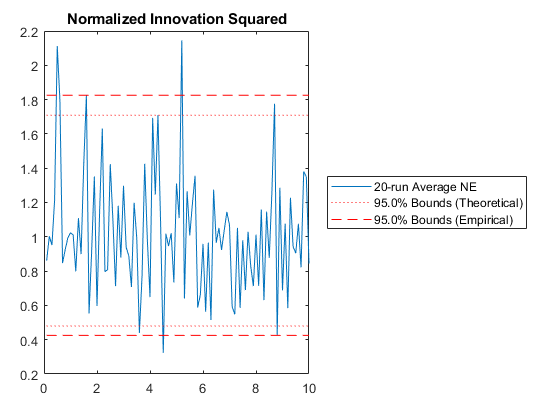
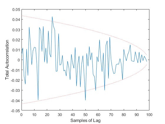
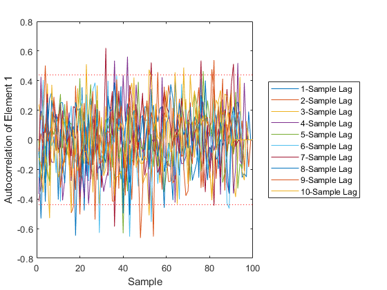
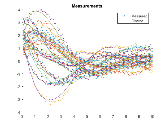
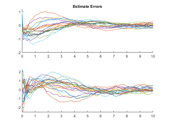
kffmct(nr, ts, dt, xh0, P0, Pxc0, ufcn, f, Fc, Q, h, Hc, R, Pc, opt);

This function by default produces several plots of the results, including the states, measurements, and statistical properties of the errors.

Inputs

 u_km1 = u_fcn(t_km1, x_hat_km1, (etc.));

Outputs

Option-Value Pairs

 kffmct(..., 'UserVars', {arg1, arg2});

 1: States and estimates                                  
 2: Measurements and filtered measurements                
 3: Estimate errors                                       
 4: Normalized estimation error squared                   
 5: Normalized mean estimation error                      
 6: Normalized innovation squared                         
 7: Total residual autocorrelation                        
 8: Innovation autocorrelation                            

 kffmct(1, ..., 'Seed0', 17);

 x_k = f(t_km1, t_k, x_km1, u_km1, c);                    
 z_k = h(t_k, x_km1, u_km1, c);                           

Example of a Linear System

Let's use the kff to filter a perfectly linear system.

Define a system.

dt    = 0.1;                                  % Time step
F_km1 = expm([0 1; -1 0]*dt);                 % State transition matrix
H_k   = [1 0];                                % Observation matrix
Q_km1 = 0.5^2 * [0.5*dt^2; dt]*[0.5*dt^2 dt]; % Process noise covariance
R_k   = 0.1^2;                                % Meas. noise covariance

Set some simulation options.

% Set the initial conditions.
x_hat_0 = [1; 0];                    % Initial estimate
P_0     = diag([0.5 1].^2);          % Initial estimate covariance
 
% Define things for kff.
f = @(t0, tf, x, u) F_km1 * x;
h = @(t, x, u) x(1);
options = kffoptions('F_km1_fcn',   F_km1, ...
                     'Q_km1_fcn',   Q_km1, ...
                     'H_k_fcn',     H_k, ...
                     'R_k_fcn',     R_k, ...
                     'f',           f, ...
                     'h',           h, ...
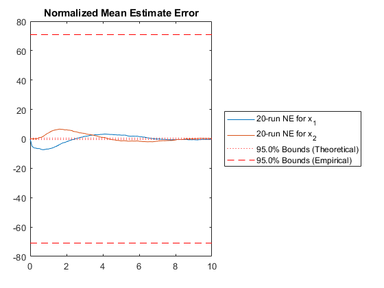
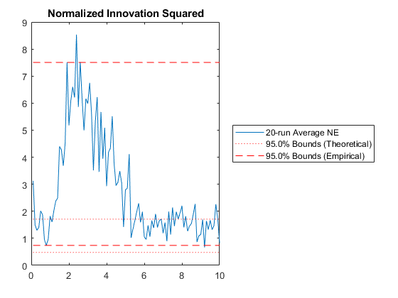
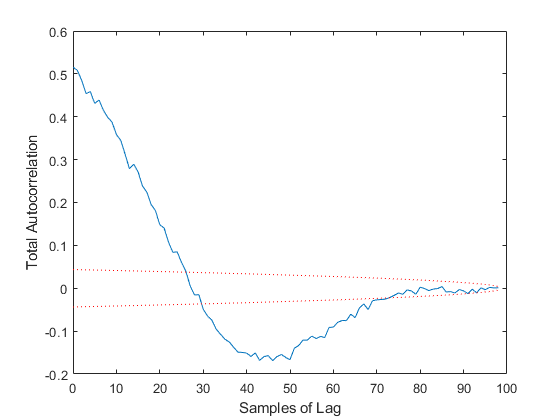
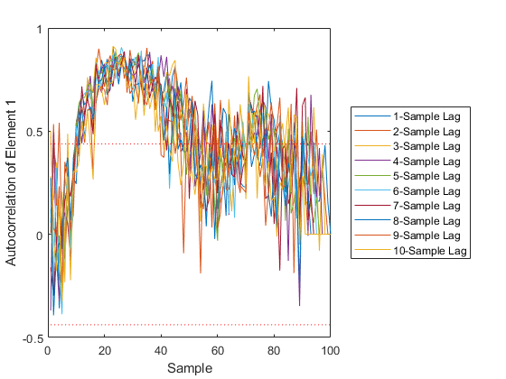
                     'joseph_form', false);

Run 20 simulations with different random draws, and then show statistics.

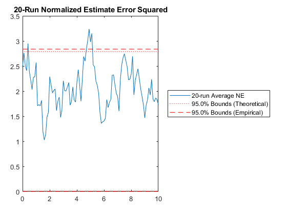
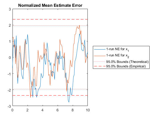
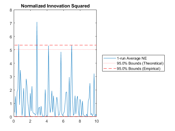
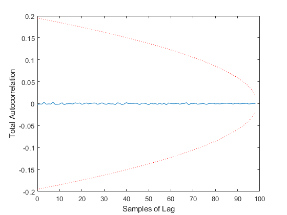
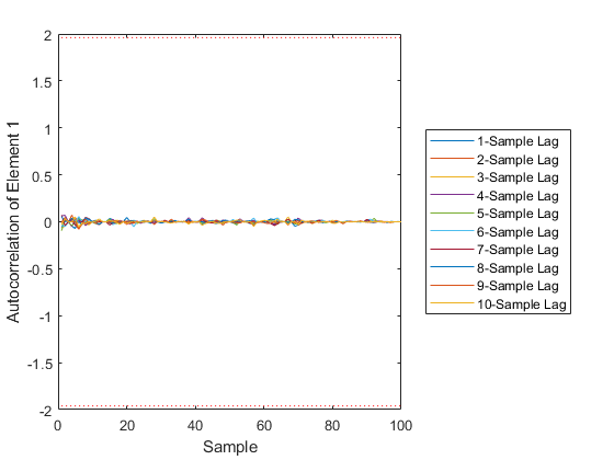
kffmct(20, [0 10], dt, x_hat_0, P_0, options);

NEES: Percent of data in theoretical 95.0% bounds: 94.1%
NMEE: Percent of data in theoretical 95.0% bounds: 98.0%
NIS:  Percent of data in theoretical 95.0% bounds: 91.0%
TAC:  Percent of data in theoretical 95.0% bounds: 94.9%
AC:   Percent of data in theoretical 95.0% bounds: 95.8%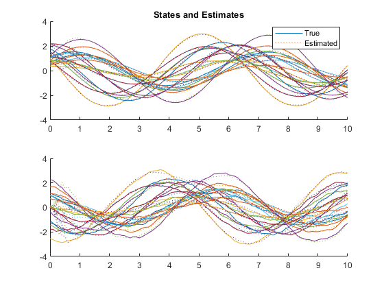

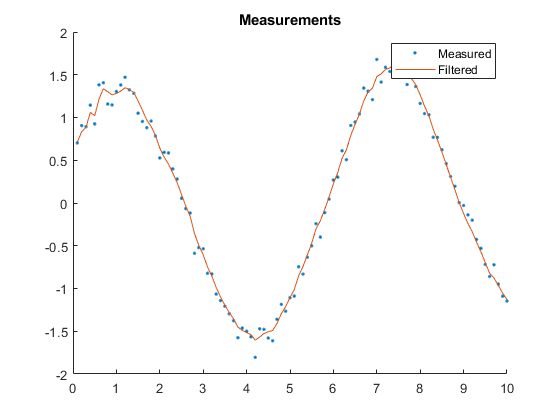
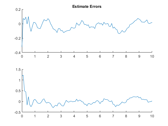
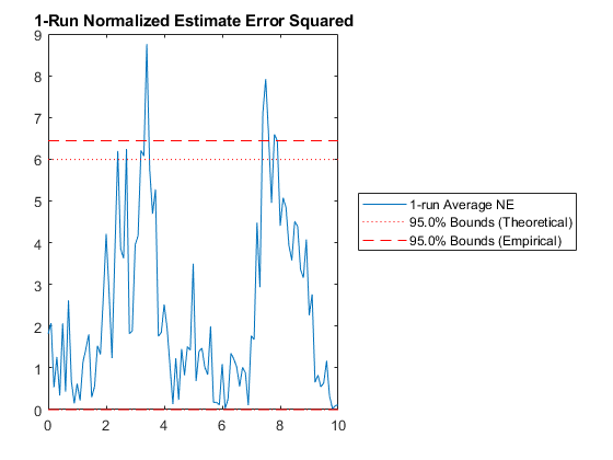
Of course, we can use kffmct to simulate a single run too.

kffmct(1, [0 10], dt, x_hat_0, P_0, options);

NEES: Percent of data in theoretical 95.0% bounds: 90.1%
NMEE: Percent of data in theoretical 95.0% bounds: 93.6%
NIS:  Percent of data in theoretical 95.0% bounds: 95.0%
TAC:  Percent of data in theoretical 95.0% bounds: 100.0%
AC:   Percent of data in theoretical 95.0% bounds: 100.0%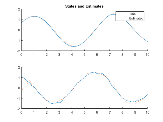

Example of Misalignment between True and Filter Models

We can also use a different model for the true f and h and see what the result is on the estimator.

f_true = @(t0, tf, x, u) expm([0 1; -0.5 -0.5] * dt) * x; % Different!
h_true = @(t, x, u) 1.5 * x(1);                           % Also different
Q_true = Q_km1;
R_true = R_k;
 
% Run 20 sims to see how things look.
kffmct(20, [0 10], dt, x_hat_0, P_0, [], ...
       f_true, Q_true, h_true, R_true, options);

NEES: Percent of data in theoretical 95.0% bounds: 1.0%
NMEE: Percent of data in theoretical 95.0% bounds: 23.3%
NIS:  Percent of data in theoretical 95.0% bounds: 41.0%
TAC:  Percent of data in theoretical 95.0% bounds: 28.3%
AC:   Percent of data in theoretical 95.0% bounds: 42.0%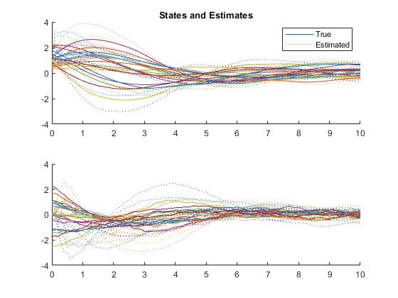

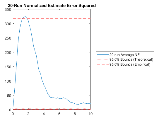
Few points are within the bounds predicted by the estimate covariance, suggesting that the filter is missing some important part of the true system and that our filter is, as a result, too optimistic. We could either figure out more about the true system, where that's feasible, or using consider covariance to represent additional uncertainty in the model.

See Also

kff, kffoptions