by An Uncommon Lab

Homework 2, Answer 2: The *kf Engine Method

This script shows how to create a filter, simulaiton, and Monte-Carlo test for homework problem 2 using the *kf engine. Several additional files are part of this solution as well, and will be shown below.

To work with this solution, use the following to copy the various solution files to your current directory:

skfexample('hw2ans2');

Define the System

We'll begin with the constants described in homework 2.

% Basic constants
u = 1;   % Generalized application force
a = 0.1; % Constant mapping generalized force to generalized pressure
 
% Initial conditions
P_0     = (0.05)^2 * eye(3);
x_hat_0 = [0; 0; 0];
 
% Measurement noise covariance
R = 0.003^2 * eye(3);

Propagation Function

We have all of the necessary functions implemented in their own files. Here is the propagation function.

type propagate;

 
function x_k = propagate(t_km1, t_k, x_km1, u_km1, a) %#ok
 
% propagate
% 
% Update the state from sample k-1 to sample k. This function is discrete
% and doesn't actually use the time inputs.
 
    p   = a * u_km1/(sum(x_km1) + 3);       % Generalized pressure
    x_k = x_km1 - p * x_km1 ./ (x_km1 + 1); % Vectorized calculation
 
end % propagate

Jacobian of the Propagation Function

type F_fcn;

 
function F = F_fcn(t_km1, t_k, x, u, a) %#ok
 
% F_fcn
% 
% Calculate the Jacobian of the propagation function wrt the state.
 
    % Calculate the generalized pressure term.
    p = a * u/(sum(x) + 3);
    
    % Differentiate the pressure wrt x1, x2, or x3 (it's the same
    % regardless of which element of x is used).
    dpdxi = -p/(sum(x) + 3);
    
    % Differentiate the first element of the propagation function, f, by x2
    % or x3; it will be the same for either. Repeat for f2 wrt x1 or x3 and
    % f3 wrt x1 or x2.
    df1dxi = -dpdxi * x(1)/(x(1) + 1);
    df2dxi = -dpdxi * x(2)/(x(2) + 1);
    df3dxi = -dpdxi * x(3)/(x(3) + 1);
    
    % Differentiate f1 wrt x1. Part of this is the same as df1/dx2 or 
    % df1/dx3, plus a 1 and a pressure term.
    df1dx1 = 1 + df1dxi - p / (x(1) + 1)^2;
    df2dx2 = 1 + df2dxi - p / (x(2) + 1)^2;
    df3dx3 = 1 + df3dxi - p / (x(3) + 1)^2;
    
    % Build the final Jacobian.
    F = [df1dx1, df1dxi, df1dxi; ...
         df2dxi, df2dx2, df2dxi; ...
         df3dxi, df3dxi, df3dx3];
 
end % F_fcn

Before we go any further, let's test the Jacobian at some random point drawn from P_0.

x_test = mnddraw(P_0);
F_fcn(0, 1, x_test, u, a)
fdiff(@propagate, ...       Function that we should differentiate
      1e-6, ...             Step size to use for differentiation
      3, ...                x is the 3rd argument to the propagate function
      0, 1, x_test, u, a) % Arguments to the propagate function

ans =
    0.9658   -0.0001   -0.0001
    0.0004    0.9689    0.0004
   -0.0008   -0.0008    0.9608
ans =
    0.9658   -0.0001   -0.0001
    0.0004    0.9689    0.0004
   -0.0008   -0.0008    0.9608

Looks good.

Process Noise

type Q_fcn;

 
function Q = Q_fcn(t_km1, t_k, x, u, a) %#ok
 
% Q_fcn
%
% Calculate the process noise. When there's more build-up, there's more
% process noise, as described in hw2.m.
 
    Q = diag(1e-4 + 1e-2 * x.^2);
 
end % Q_fcn

Observation Function

type observe;

 
function z = observe(t, x, u, a) %#ok
 
% observe
% 
% Create the observation vector based on the current state and input.
 
    % Generalized pressure
    p = a * u/(sum(x) + 3);
    
    % Generalized pressure maps the state to the measurement directly.
    z = p * x;
 
end % observe

Jacobian of the Observation Function

type H_fcn;

 
function H = H_fcn(t, x, u, a) %#ok
 
% H_fcn
% 
% Create the Jacobian of the observation function.
 
    H = a*u/(sum(x) + 3)^2 * ...
            [x(2)+x(3)+3,       -x(1),       -x(1); ...
                   -x(2), x(1)+x(3)+3,       -x(2); ...
                   -x(3),       -x(3), x(1)+x(2)+3];
 
end % H_fcn

Let's test this Jacobian too. We'll use the same test point as before.

H_fcn(0, x_test, u, a)
fdiff(@observe, ...      Function to differentiate
      1e-6, ...          Step size
      2, ...             x is the 2nd input to the observe function.
      0, x_test, u, a) % Arguments to the observe function

ans =
    0.0338    0.0001    0.0001
   -0.0004    0.0333   -0.0004
    0.0007    0.0007    0.0344
ans =
    0.0338    0.0001    0.0001
   -0.0004    0.0333   -0.0004
    0.0007    0.0007    0.0344

Looks good.

Set the *kf Options

We could use skfengine to open the graphical user interface and enter all of the necessary values by hand. Or, we could use the skfoptions struct and just change the defaults that we care about. We'll do the latter, but after we've set things up, we'll open the GUI just to check that we've done things correctly.

% Create the default options.
options = skfoptions();
 
% Set up the basic filter stuff. When telling the *kf engine to use a
% variable in the workspace, we pass in a string so that it knows what
% variable to look for.
options.filter_name           = 'hw2ans2';
options.init.x0               = 'x_hat_0';
options.init.uncertainty.type = 'Covariance'; % (default)
options.init.uncertainty.P0   = 'P_0';
options.inputs.z_example      = '[0; 0; 0]';
options.inputs.u_example      = '1'; % Will be a constant in the sim.
options.filter_type           = 'Linear'; % (default)
options.inputs.additional_inputs = 'a'; % We'll use 'a' everywhere.
 
% Set up the propagation-related options to use a nonlinear system with
% system matrices determine from the current state estimate, yielding an
% extended Kalman filter.
options.dkf.prop_type          = 'Nonlinear'; % Nonlinear propagation fcn
options.dkf.f                  = 'propagate';
options.dkf.F.type             = 'Function';  % Jacobian of f wrt x
options.dkf.F.fcn              = 'F_fcn';
options.dkf.Q.type             = 'Function';  % Process noise covariance
options.dkf.Q.fcn              = 'Q_fcn';
options.dkf.include_input_in_f = true;        % We use an input vector.
 
% Set the observation function, observation Jacobian function, and constant
% measurement noise covariance.
options.dkf.obs_type           = 'Nonlinear'; % Nonlinear observation fcn
options.dkf.h                  = 'observe';
options.dkf.H.type             = 'Function';  % Jacobian of h wrt x
options.dkf.H.fcn              = 'H_fcn';
options.dkf.R.type             = 'Constant';  % Meas. noise covariance
options.dkf.R.value            = 'R';
options.dkf.include_input_in_h = true;        % Observation uses the input.
 
% Let's set up the test options to give us a 30 second run.
options.test.time_step = 1;
options.test.num_steps = 300;
options.test.num_runs  = 100;
 
% Add a custom comment.
options.output.header_comments = {'Homework 2: Nozzle build-up estimator'};

Take a Look at the Setup

We'll open the *kf engine GUI and look at what we've set to make sure it looks good.

skfengine(options);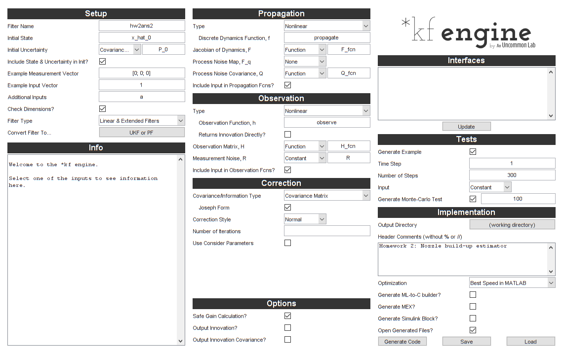

Generate Code

It looks right. Let's generate the code.

skfgen(options);

Generating code for hw2ans2.
Successfully generated code for hw2ans2.

Let's take a look at our generated filter.

type hw2ans2_step.m

 
function [x, P] = hw2ans2_step(t_km1, t_k, x, P, u_km1, z_k, constants, user_a)
 
% hw2ans2_step
% 
% Homework 2: Nozzle build-up estimator
% 
% Inputs: 
% 
% t_km1         Time at sample k-1
% t_k           Time at sample k
% x             Estimated state at k-1 (prior)
% P             Estimate covariance at k-1 (prior)
% u_km1         Input vector at sample k-1
% z_k           Measurement at k
% constants     Constants struct from initialization function
% user_a        User-defined variable 1
% 
% Outputs: 
% 
% x             Estimated state at sample k
% P             Estimate error covariance at sample k
% 
% Generated with *kf v1.0.3
 
    %#codegen
 
    % Tell MATLAB Coder how to name the constants struct.
    coder.cstructname(constants, 'hw2ans2_constants');
 
    % See if we need to propagate.
    if t_k > t_km1
 
        % Create the Jacobian of the propagation function wrt the state.
        F_km1 = F_fcn(t_km1, t_k, x, u_km1, user_a);
 
        % Create the process noise covariance matrix.
        Q_km1 = Q_fcn(t_km1, t_k, x, u_km1, user_a);
 
        % Linearly propagate the covariance.
        P = F_km1 * P * F_km1.' + Q_km1;
 
        % Propagate the state.
        x = propagate(t_km1, t_k, x, u_km1, user_a);
 
    end % propagation frame
 
    % Create the observation matrix.
    H_k = H_fcn(t_k, x, u_km1, user_a);
 
    % Predict the measurement.
    z_hat_k = observe(t_k, x, u_km1, user_a);
 
    % Innovation vector at sample k
    y_k = z_k - z_hat_k;
 
    % State-measurement covariance at k
    P_xy_k = P * H_k.';
 
    % Innovation covariance matrix at k (local)
    P_yy_k = H_k * P_xy_k + constants.R_k;
 
    % Safely calculate the Kalman gain.
    K = smrdivide(P_xy_k, P_yy_k);
 
    % Update the state estimate.
    x = x + K * y_k;
 
    % Build the matrix used for Joseph form covariance correction.
    A = -K * H_k;
    A = addeye(A);
 
    % Update the estimate covariance (Joseph form).
    P = A * P * A.';
    P = P + K * constants.R_k * K.';
 
end % hw2ans2_step
 

Run the Simulation and Monte-Carlo Test

We can now run the generated simulation. Note that we said that a should be an additional argument to the filter, so we'll need to pass it in here. The example will pass it on to the filter.

hw2ans2_example(a);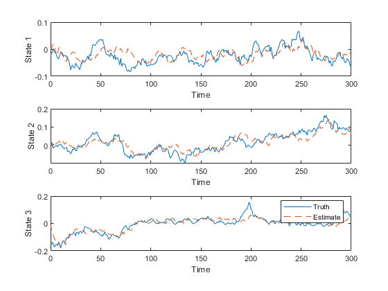

Since that looks good, here are the Monte-Carlo test results.

hw2ans2_mc(a);

NEES: Percent of data in theoretical 95.0% bounds: 73.1%
NMEE: Percent of data in theoretical 95.0% bounds: 91.7%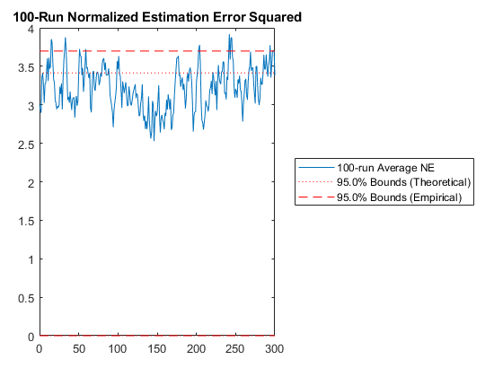

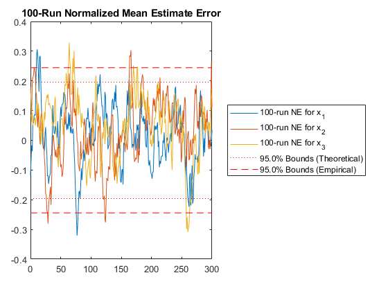
The normalized estimation error squared statistic is a little low, but the homework said to expect this for this application, so we're done with this problem.