
hw2ans1
function hw2ans1()
% hw2ans1
%
% This function demonstrates how to solve homework problem 2 using the
% Kalman Filter Framework tools. All of the work is contained in this
% single file, showing how quickly one can use kff to create a filter
% prototype.
%
% See skfexample('hw2') for more.
% Copyright 2016 An Uncommon Lab
% Set up the initial conditions directly from hw1.m.
P_0 = (0.05)^2 * eye(3);
x_hat_0 = [0; 0; 0];
% Set up some constants related to the dynamics.
dt = 1; % We update discretely; let dt be 1 for "one step".
u = 1; % Generalized application force
a = 0.1; % Constant mapping generalized force to generalized pressure
% The only constant for this filter is the measurement noise
% covariance.
R = 0.003^2 * eye(3);
% Set up the options for kff, telling it which functions to call for
% propagation, observation, process noise, and the various Jacobians.
options = kffoptions('f', @propagate, ...
'F_km1_fcn', @propagation_jacobian, ...
'Q_km1_fcn', @process_noise, ...
'h', @observe, ...
'H_k_fcn', @observation_jacobian, ...
'R_k_fcn', R);
% Run a simulation for 300 applications. Pass our 'a' variable along to
% each function that kff calls as well (the functions below use 'a').
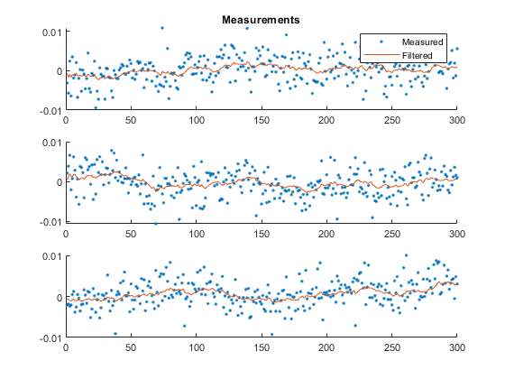
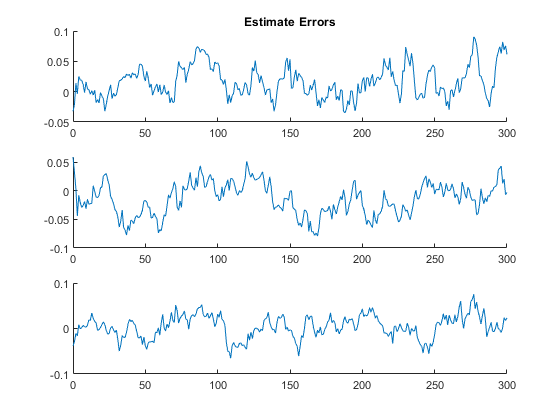
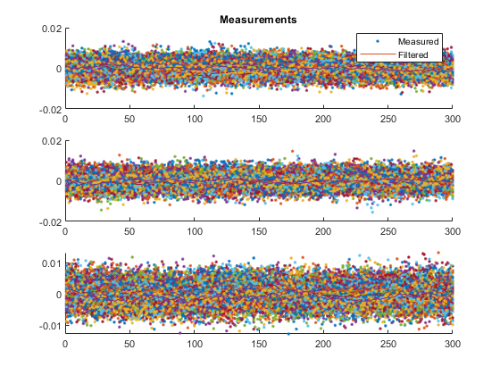
kffsim([0, 300], dt, x_hat_0, P_0, u, options, ...
'UserVars', {a});
snapnow();
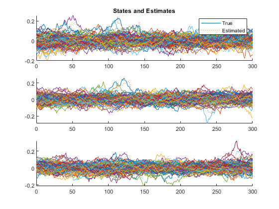
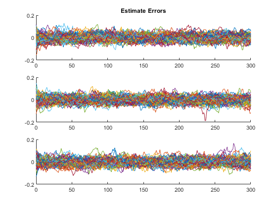
% Run a Monte-Carlo test with 100 simulations for 300 applications
% each.
kffmct(100, [0 300], dt, x_hat_0, P_0, u, options, 'UserVars', {a});
end % hw2ans1
% Update the state from sample k-1 to sample k. This function is discrete
% and doesn't actually use the time inputs.
function x_k = propagate(t_km1, t_k, x_km1, u_km1, a) %#ok
p = a * u_km1/(sum(x_km1) + 3); % Generalized pressure
x_k = x_km1 - p * x_km1 ./ (x_km1 + 1); % Vectorized calculation
end % propagate
% Calculate the Jacobian of the propagation function wrt the state.
function F = propagation_jacobian(t_km1, t_k, x, u, a) %#ok
% Calculate the generalized pressure term.
p = a * u/(sum(x) + 3);
% Differentiate the pressure wrt x1, x2, or x3 (it's the same
% regardless of which element of x is used).
dpdxi = -p/(sum(x) + 3);
% Differentiate the first element of the propagation function, f, by x2
% or x3; it will be the same for either. Repeat for f2 wrt x1 or x3 and
% f3 wrt x1 or x2.
df1dxi = -dpdxi * x(1)/(x(1) + 1);
df2dxi = -dpdxi * x(2)/(x(2) + 1);
df3dxi = -dpdxi * x(3)/(x(3) + 1);
% Differentiate f1 wrt x1. Part of this is the same as df1/dx2 or
% df1/dx3, plus a 1 and a pressure term.
df1dx1 = 1 + df1dxi - p / (x(1) + 1)^2;
df2dx2 = 1 + df2dxi - p / (x(2) + 1)^2;
df3dx3 = 1 + df3dxi - p / (x(3) + 1)^2;
% Build the final Jacobian.
F = [df1dx1, df1dxi, df1dxi; ...
df2dxi, df2dx2, df2dxi; ...
df3dxi, df3dxi, df3dx3];
end % propagation_jacobian
% Calculate the process noise. When there's more build-up, there's more
% process noise, as described in hw2.m.
function Q = process_noise(t_km1, t_k, x, u, a) %#ok
Q = diag(1e-4 + 1e-2 * x.^2);
end % process_noise
% Create the observation vector based on the current state and input.
function z = observe(t, x, u, a) %#ok
% Generalized pressure
p = a * u/(sum(x) + 3);
% Generalized pressure maps the state to the measurement directly.
z = p * x;
end % observe
% Create the Jacobian of the observation function.
function H = observation_jacobian(t, x, u, a) %#ok
H = a*u/(sum(x) + 3)^2 * ...
[x(2)+x(3)+3, -x(1), -x(1); ...
-x(2), x(1)+x(3)+3, -x(2); ...
-x(3), -x(3), x(1)+x(2)+3];
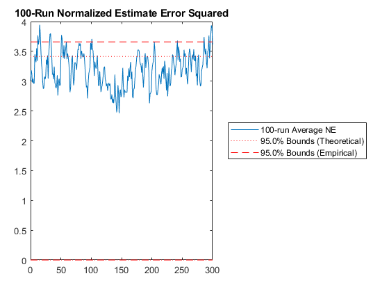
end % observation_jacobian ml2jade1Z2Xml2jade1A6XNEES: Percent of data in theoretical 95.0% bounds: 75.7%
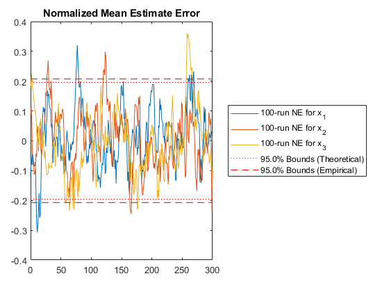
NMEE: Percent of data in theoretical 95.0% bounds: 93.6%
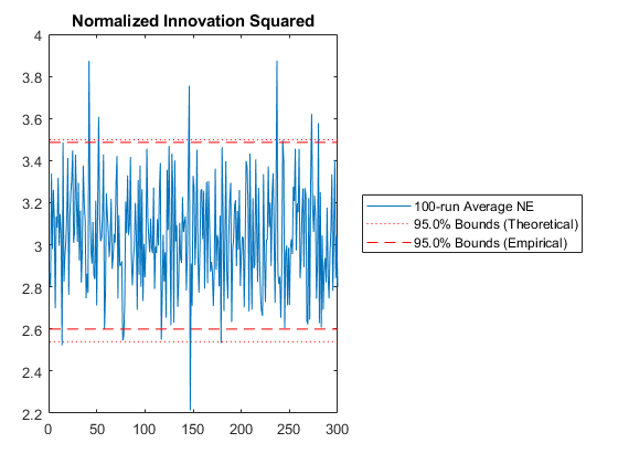
NIS: Percent of data in theoretical 95.0% bounds: 97.0%
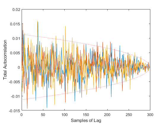
TAC: Percent of data in theoretical 95.0% bounds: 95.1%
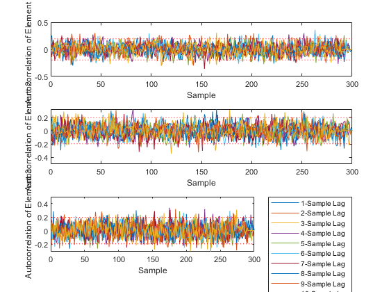
AC: Percent of data in theoretical 95.0% bounds: 94.9%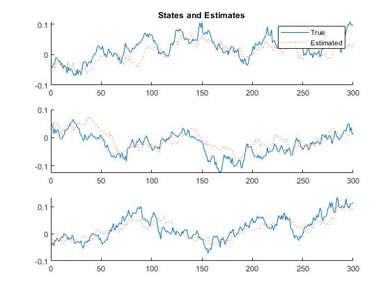
*kf v1.0.3 January 17th, 2025
©2025 An Uncommon Lab