
hw1ans3
function hw1ans3()
% Homework 1, Answer 3: The Basic Filter Method
%
% This function solves homework problem 1 using one of the "basic filters".
% It requires that we construct the simulation and Monte-Carlo loops
% directly, but is still pretty easy since this is a linear problem.
%
% See skfexample('hw1') for more.
% Copyright 2016 An Uncommon Lab
% Constants for the dynamics
dt = 0.25; % Time step [s]
m = 10; % Mass [kg]
k = 5; % Spring constant [N/m]
b = 2; % Spring damping [N/(m/s)]
% Continuous-time Jacobian for the linear system: x_dot = A * x
A = [0 1; -k/m, -b/m];
% Discrete-time Jacobian: x_k = F * x_km1
F = expm(A * dt);
% The process noise consists of a single acceleration parameter, q.
% This acceleration maps to the change in position and velocity as:
%
% dp = 0.5 * dt^2 * q
% dv = dt * q
%
% Or, using the state vector x = [p; v]:
%
% dx = [0.5 * dt^2; dt] * q = Fq * q
%
% The covariance of dx is (using E(.) as the expectation operator):
%
% E(dx * dx.') = E(Fq * q * q.' * Fq.')
% = Fq * E(q*q.') * Fq.'
% = Fq * Q * Fq.'
%
% where Q is the given process noise variance (0.1 m/s^2)^2.
%
Q = 0.1^2;
Fq = [0.5*dt^2; dt];
Qe = Fq * Q^2 * Fq.';
% We observe the position only.
H = [1 0];
% The measurement noise variance is given as m^2.
R = 0.1^2;
% The initial estimate and covariance are given.
x_hat_0 = [1; 0]; % [m, m/s]
P_0 = diag([1 2]); % [m^2, m^2/s^2]
% Create the initial true state from the initial estimate and
% covariance.
x_0 = x_hat_0 + mnddraw(P_0);
% Create the time histories.
t = 0:dt:30;
n = length(t);
x = [x_0, zeros(2, n-1)];
x_hat = [x_hat_0, zeros(2, n-1)];
P = cat(3, P_0, zeros(2, 2, n-1));
% Simulate to the 30s end time.
for k = 2:n
% Update the truth.
x(:, k) = F * x(:, k-1) + Fq * mnddraw(Q);
% Create the measurement.
z = x(1, k) + mnddraw(R);
% Run the linear filter for a single step.
[x_hat(:, k), P(:, :, k)] = lkf(x_hat(:, k-1), P(:, :, k-1), ...
[], z, F, [], H, Qe, R);
end % sim loop
% Plot the results to make sure things look good.
unique_figure(mfilename());
subplot(2, 1, 1);
plot(t, x(1, :), t, x_hat(1, :));
ylabel('Position');
subplot(2, 1, 2);
plot(t, x(2, :), t, x_hat(2, :));
ylabel('Velocity');
% Do the above for 100 runs for a Monte-Carlo test.
m = 100;
errs_mc = zeros(2, n, m);
P_mc = zeros(2, 2, n, m);
for r = 1:m
% Create the initial true state.
x_0 = x_hat_0 + mnddraw(P_0);
% Create the histories for this run.
x = [x_0, zeros(2, n-1)];
x_hat = [x_hat_0, zeros(2, n-1)];
P = cat(3, P_0, zeros(2, 2, n-1));
% Simulate to the 30s end time.
for k = 2:n
% Update the truth.
x(:, k) = F * x(:, k-1) + Fq * mnddraw(Q);
% Create the measurement.
z = x(1, k) + mnddraw(R);
% Run the linear filter for a single step.
[x_hat(:, k), P(:, :, k)] = lkf(x_hat(:, k-1), P(:, :, k-1), ...
[], z, F, [], H, Q, R);
end % sim loop
% Record the errors and covariance.
errs_mc(:, :, r) = x - x_hat;
P_mc(:, :, :, r) = P;
end % mc loop
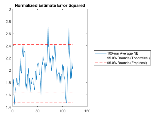
% Plot the normalized estimation error squared.
unique_figure([mfilename() ':NEES']);
normerr(errs_mc, P_mc, 0.95, 1);
title('Normalized Estimate Error Squared');
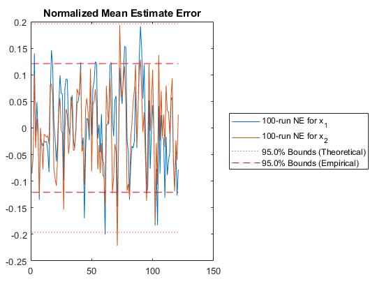
% Plot the normalized mean estimate error.
unique_figure([mfilename() ':NMEE']);
normerr(errs_mc, P_mc, 0.95, 2);
title('Normalized Mean Estimate Error');
end % hw1ans3Percent of data in theoretical 95.0% bounds: 89.3%
Percent of data in theoretical 95.0% bounds: 99.2%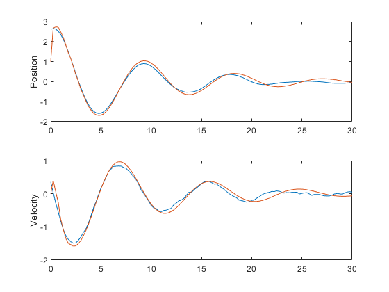
*kf v1.0.3 January 17th, 2025
©2025 An Uncommon Lab