by An Uncommon Lab

Homework 1, Answer 2: The *kf Engine Method

This file shows how to create a filter with a simulation and Monte-Carlo test for homework problem 1 using the *kf engine.

Define the System

We'll define the system directly based on the description in homework 1.

% Constants for the dynamics
dt = 0.25; % Time step [s]
m  = 10;   % Mass [kg]
k  = 5;    % Spring constant [N/m]
b  = 2;    % Spring damping  [N/(m/s)]
 
% Continuous-time Jacobian for the linear system: x_dot = A * x
A = [0 1; -k/m, -b/m];
 
% Discrete-time Jacobian for the linear system: x_k = F * x_km1
F = expm(A * dt);
 
% Process noise
Q = 0.1^2;
 
% Process noise map
Fq = [0.5*dt^2; dt];
 
% The measurement noise variance is given as m^2.
R = 0.1^2;
 
% The initial estimate and covariance are given.
x_hat_0 = [1; 0];      % [m,   m/s]
P_0     = diag([1 2]); % [m^2, m^2/s^2]

Set the *kf Options

We could use skfengine to open the graphical user interface and enter all of the necessary values by hand. Or, we could use the skfoptions struct and just change the defaults that we care about. We'll do the latter, but after we've set things up, we'll open the GUI just to check that we've done things correctly.

% Create the default options.
options = skfoptions();
 
% Set up the basic filter stuff. When telling the *kf engine to use a
% variable in the workspace, we pass in a string so that it knows what
% variable to look for.
options.filter_name           = 'hw1ans2';
options.init.x0               = 'x_hat_0';
options.init.uncertainty.type = 'Covariance'; % (default)
options.init.uncertainty.P0   = 'P_0';
options.inputs.z_example      = '0';
options.filter_type           = 'Linear'; % (default)
 
% Set up the propagation-related options to use a linear system with
% constant system matrices and no input vector.
options.dkf.prop_type          = 'Linear';
options.dkf.F.type             = 'Constant'; % Jacobian of f wrt x
options.dkf.F.value            = 'F';
options.dkf.F_q.type           = 'Constant'; % Jacobian of f wrt q
options.dkf.F_q.value          = 'Fq';
options.dkf.Q.type             = 'Constant'; % Process noise covariance
options.dkf.Q.value            = 'Q';
options.dkf.include_input_in_f = false;      % We don't use a u vector.
 
% For the observation, we could define an observation function or use a
% linear observation function, but the fastest thing for our filter is to
% use the "subset" option. This says that the observation is actually just
% a subset of the state (it's index 1 of the state). When we do this, we
% won't need a Jacobian of the observation function (which would just be
% [1 0]).
options.dkf.obs_type  = 'Subset';
options.dkf.h_indices = '1';
options.dkf.R.type    = 'Constant'; % Measurement noise covariance
options.dkf.R.value   = 'R';
 
% Let's set up the test options to give us a 30 second run.
options.test.time_step = 'dt';
options.test.num_steps = 30/dt;
options.test.num_runs  = '100';

Take a Look at the Setup

We'll open the *kf engine GUI and look at what we've set to make sure it looks good.

skfengine(options);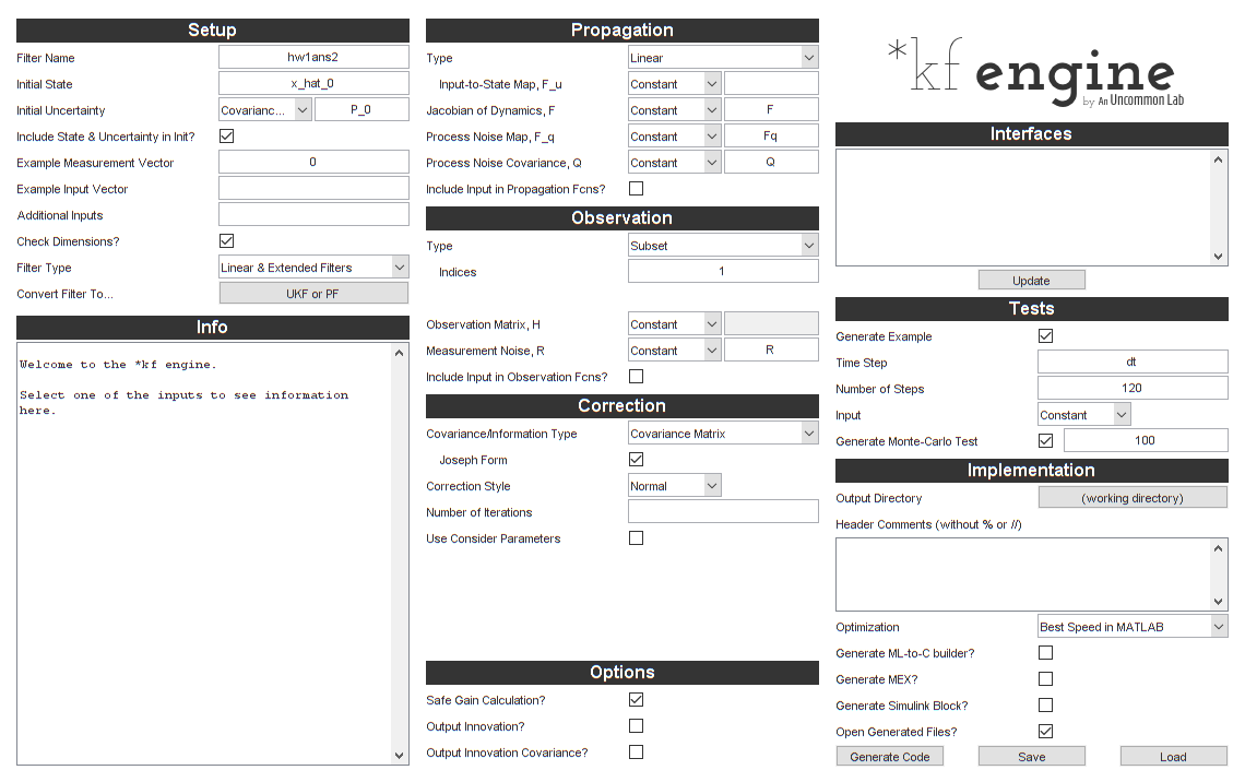

Generate Code

It looks right. Let's generate the code.

skfgen(options);

Generating code for hw1ans2.
[Warning: Class 'SkfFrame' uses an undocumented syntax to restrict
property values. Use property validation syntax instead. This warning
will become an error in a future release.] 
[> In make_lin_propagation (line 16)
In make_lin_step (line 152)
In code_lin (line 201)
In skfgen (line 43)
In ml2jade (line 254)
In enjaden (line 360)
In deploy_web>do_tutorial (line 130)
In deploy_web (line 107)] 
[Warning: Class 'SkfMemory' uses an undocumented syntax to restrict
property values. Use property validation syntax instead. This warning
will become an error in a future release.] 
[> In SkfFunction/make (line 121)
In make_lin_step (line 255)
In code_lin (line 201)
In skfgen (line 43)
In ml2jade (line 254)
In enjaden (line 360)
In deploy_web>do_tutorial (line 130)
In deploy_web (line 107)] 
Successfully generated code for hw1ans2.

Run the Simulation and Monte-Carlo Test

We can now run the generated simulation.

hw1ans2_example();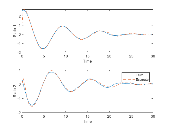

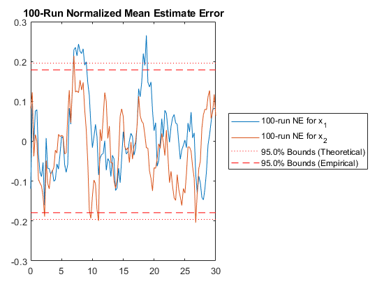
Since that looks good, here are the Monte-Carlo test results.

hw1ans2_mc();

NEES: Percent of data in theoretical 95.0% bounds: 91.7%
NMEE: Percent of data in theoretical 95.0% bounds: 94.6%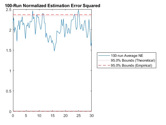

Let's take a look at our generated filter.

type hw1ans2_step.m

 
function [x, P] = hw1ans2_step(t_km1, t_k, x, P, z_k, constants)
 
% hw1ans2_step
% 
% Inputs: 
% 
% t_km1         Time at sample k-1
% t_k           Time at sample k
% x             Estimated state at k-1 (prior)
% P             Estimate covariance at k-1 (prior)
% z_k           Measurement at k
% constants     Constants struct from initialization function
% 
% Outputs: 
% 
% x             Estimated state at sample k
% P             Estimate error covariance at sample k
% 
% Generated with *kf v1.0.3
 
    %#codegen
 
    % Tell MATLAB Coder how to name the constants struct.
    coder.cstructname(constants, 'hw1ans2_constants');
 
    % Indices of the state that are directly observed
    z_ind = 1;
 
    % Dimension of the state
    nx = length(x);
 
    % See if we need to propagate.
    if t_k > t_km1
 
        % Linearly propagate the covariance.
        P = constants.F_km1 * P * constants.F_km1.' + constants.Q_eff;
 
        % Estimated state at k based on information from k-1 (prior)
        x = constants.F_km1 * x;
 
    end % propagation frame
 
    % Predict the measurement.
    z_hat_k = x(z_ind);
 
    % Innovation vector at sample k
    y_k = z_k - z_hat_k;
 
    % State-measurement covariance at k
    P_xy_k = P(:, z_ind);
 
    % Innovation covariance matrix at k (local)
    P_yy_k = P(z_ind, z_ind) + constants.R_k;
 
    % Safely calculate the Kalman gain.
    K = smrdivide(P_xy_k, P_yy_k);
 
    % Update the state estimate.
    x = x + K * y_k;
 
    % Build the matrix used for Joseph form covariance correction.
    A = eye(nx);
    A = assign2col(A, -K, z_ind);
 
    % Update the estimate covariance (Joseph form).
    P = A * P * A.';
    P = P + K * constants.R_k * K.';
 
end % hw1ans2_step
 

While we're at it, let's take a look at the initialization file:

type hw1ans2_init.m

 
function [x_0, P_0, constants] = hw1ans2_init()
 
% hw1ans2_init
% 
% Initialization for hw1ans2_step().
% 
% Inputs: 
% 
% 
% 
% Outputs: 
% 
% x_0           Initial state estimate
% P_0           Initial estimate covariance
% constants     Constants struct from initialization function
% 
% Generated with *kf v1.0.3
 
    %#codegen
 
    % Initial state estimate
    x_0 = [1;0];
 
    % Initial estimate covariance
    P_0 = [1 0;0 2];
 
    % Jacobian of discrete dynamics wrt the state at k-1
    constants.F_km1 = [0.984672038654168 0.242584846228324;-0.121292423114162 0.936155069408503];
 
    % Effective process noise covariance matrix
    constants.Q_eff = [9.765625e-06 7.8125e-05;7.8125e-05 0.000625];
 
    % Measurement noise covariance matrix at k
    constants.R_k = 0.01;
 
    % Name the constants struct for the sake of code generation.
    coder.cstructname(constants, 'hw1ans2_constants');
 
end % hw1ans2_init

Note that it creates the “effective process noise” for us as a constant, which is more efficient for the filter. There are many such niceties in the code, even for such a basic filter.

Wrap Up

That does it. Notice that this file is actually a little longer than hw1ans1.m (from skfexample('hw1ans1')). This might be the case for such small problems. The advantage is that this method gives us a custom filter that will run much faster than kff, can be used by anyone (whether they have *kf or not), and can support code generation. Further, exploring variations on the filter will be much faster with the *kf engine.

Bonus

Just for fun, let's switch to a UD filter for maximum numerical stability.

options.dkf.covariance_type = 'UDU';
 
% UD filters are almost always implemented with sequential updates, which
% uses a more efficient update to the U and D factors, so we'll add that
% too.
options.dkf.correction_type         = 'Sequential';
options.dkf.sequential_with_updates = false; % No 'updates' vector.
 
% Generate the code.
skfgen(options);

Generating code for hw1ans2.
Successfully generated code for hw1ans2.

Let's re-run the Monte-Carlo test. We should get exactly the same as above.

hw1ans2_mc();

NEES: Percent of data in theoretical 95.0% bounds: 91.7%
NMEE: Percent of data in theoretical 95.0% bounds: 94.6%

The results match, as expected.