
hw1ans1
function hw1ans1()
% Homework 1, Answer 1: The KFF Method
%
% This function solves homework problem 1 using the Kalman Filter
% Framework tools. All of the work is contained in this single file.
%
% It first defines the elements of the dynamics and observation functions
% and then sets up some options, runs the filter, and runs a Monte-Carlo
% test.
%
% See skfexample('hw1') for more.
% Copyright 2016 An Uncommon Lab
% Constants for the dynamics
dt = 0.25; % Time step [s]
m = 10; % Mass [kg]
k = 5; % Spring constant [N/m]
b = 2; % Spring damping [N/(m/s)]
% Continuous-time Jacobian for the linear system: x_dot = A * x
A = [0 1; -k/m, -b/m];
% Discrete-time Jacobian: x_k = F * x_km1
constants.F = expm(A * dt);
% The process noise consists of a single acceleration parameter, q.
% This acceleration maps to the change in position and velocity as:
%
% dp = 0.5 * dt^2 * q
% dv = dt * q
%
% Or, using the state vector x = [p; v]:
%
% dx = [0.5 * dt^2; dt] * q = Fq * q
%
% The covariance of dx is (using E(.) as the expectation operator):
%
% E(dx * dx.') = E(Fq * q * q.' * Fq.')
% = Fq * E(q*q.') * Fq.'
% = Fq * Q * Fq.'
%
% where Q is the given process noise variance (0.1 m/s^2)^2.
%
Fq = [0.5*dt^2, dt];
Q = Fq * 0.1^2 * Fq.';
% We observe the position only.
H = [1 0];
% The measurement noise variance is given as m^2.
R = 0.1^2;
% The initial estimate and covariance are given.
x_hat_0 = [1; 0]; % [m, m/s]
P_0 = diag([1 2]); % [m^2, m^2/s^2]
% Create the kff options structure.
options = kffoptions('f', @propagate, ...
'F_km1_fcn', constants.F, ...
'Q_km1_fcn', Q, ...
'h', @observe, ...
'H_k_fcn', H, ...
'R_k_fcn', R);
% Let's try a single simulation first.
[t, x, x_hat] = kffsim([0 30], dt, x_hat_0, P_0, options, ...
'UserVars', {constants});
% Plot the results to make sure things look good.
unique_figure(mfilename());
subplot(2, 1, 1);
plot(t, x(1, :), t, x_hat(1, :));
ylabel('Position');
subplot(2, 1, 2);
plot(t, x(2, :), t, x_hat(2, :));
ylabel('Velocity');
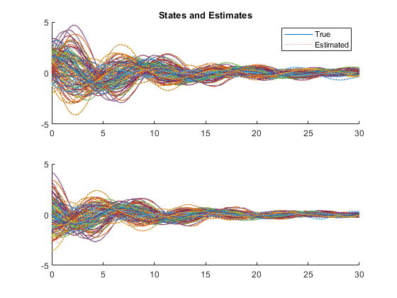
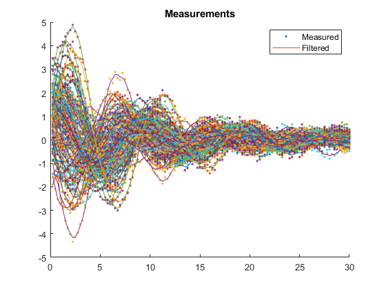
% That looks good, so let's try a Monte-Carlo test.
kffmct(100, [0 30], dt, x_hat_0, P_0, options, ...
'UserVars', {constants});
end % hw1ans1
% The propagation function is actually linear, so this part is very easy.
function x_k = propagate(t_km1, t_k, x_km1, u_km1, constants) %#ok
x_k = constants.F * x_km1;
end % propagate
% The observation function just returns the position.
function z_k = observe(t_k, x_k, u_k, constants) %#ok
z_k = x_k(1);
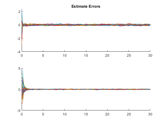
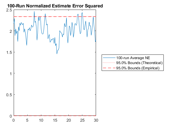
end % observe NEES: Percent of data in theoretical 95.0% bounds: 95.0%
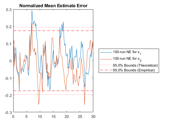
NMEE: Percent of data in theoretical 95.0% bounds: 94.6%
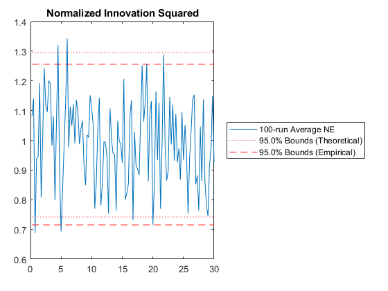
NIS: Percent of data in theoretical 95.0% bounds: 95.0%
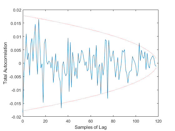
TAC: Percent of data in theoretical 95.0% bounds: 96.6%
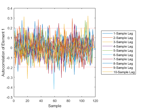
AC: Percent of data in theoretical 95.0% bounds: 95.1%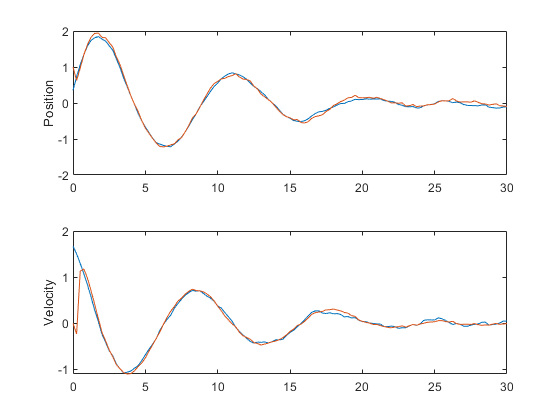
*kf v1.0.3 January 17th, 2025
©2025 An Uncommon Lab