Pendulum Tutorial: 10-Minute Introduction to the *kf Engine

This is the briefest introduction to building filters with the *kf engine. We proceed directly to building an extended Kalman filter, evaluating it, and then adding some options to improve performance. It assumes only basic knowledge about filtering.

It works like this: we tell *kf about our problem, we set a few options for the filter we want, we click Generate Code, and then we can run simulations to see how it performs. After establishing a basic filter, we can iterate on the design to improve performance.

If you have *kf installed, you can follow along with this tutorial:

skfexample('pendulum');

This will copy the example files into your local directory, so you may wish to create a new directory to work in.

If any of the language is unclear, see the nomenclature page.

Our Problem

To start, we have a propagation function and observation function defined in MATLAB as pendulum_dynamics.m and observe_pendulum.m.

For our problem, the propagation and observation functions are nonlinear, so we also have functions to calculate their Jacobians about any given state: pendulum_jacobian.m and observation_jacobian.m.

dir *.m

 
observation_jacobian.m  pendulum_dynamics.m     pendulum_tutorial.m     
observe_pendulum.m      pendulum_jacobian.m

Now we just need a few constants in order to build the filter, such as the initial state estimate:

x0 = [0; 0]; % [rad, rad/s]

the initial covariance:

P0 = diag([pi/4 pi/6].^2); % [rad^2, rad^2/s^2]

a description of the process noise:

Q  = 0.25^2; % Variance of random torques on the pendulum [Nm]
dt = 0.04;   % Time step (25Hz) [s]
m  = 1;      % Pendulum mass [kg]
r  = 0.5;    % Distance of center of mass from hinge [m]
I  = 1;      % Moment of inertia [kg m^2]
Fq = [0.5*dt^2; dt]/(I + m*r^2); % Maps torque to [angle; velocity]

and the measurement noise variance:

R  = 0.25^2 * eye(2); % [m^2]

Extended Kalman Filter

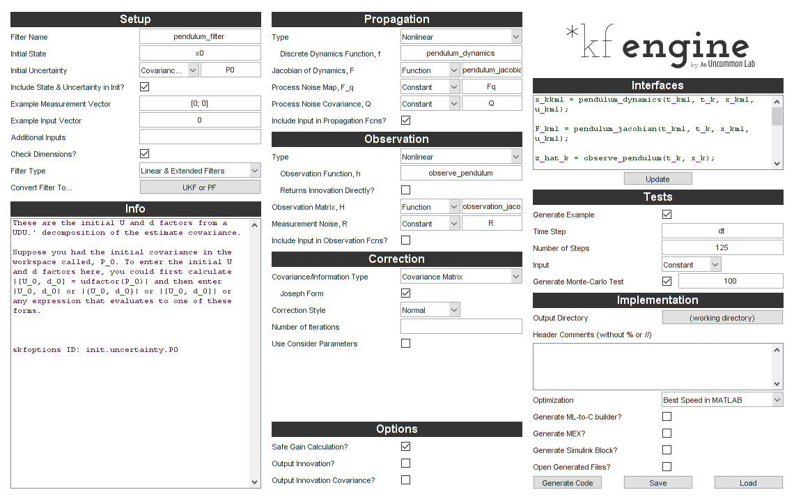
Let's open the *kf engine:

skfengine();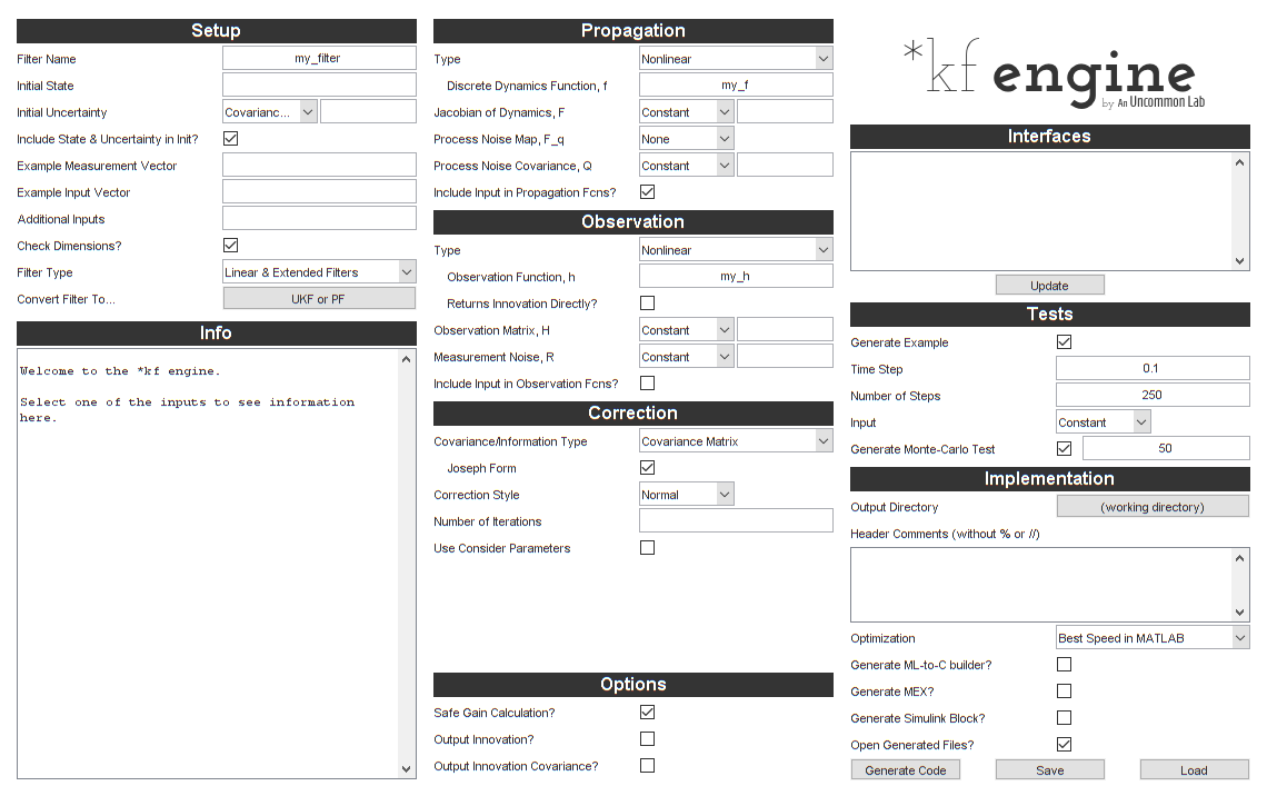

We'll start by entering a filter name and the initial values we set above. We'll also enter an example value for the measurement (a 2-by-1 for this case) and for the input vector (a scalar). This helps *kf set the dimensions appropriately in the generated filter and serves as a “sanity check” to ensure that all dimensions are consistent. We'll use a mixture of literal values (like 0) and names of variables in the base workspace (like x0).

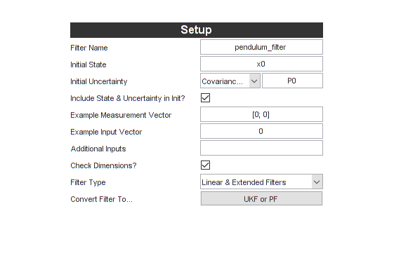
Notice that “Linear & Extended Filters” is selected by default. That's what we'll need for the extended Kalman filter we're building.

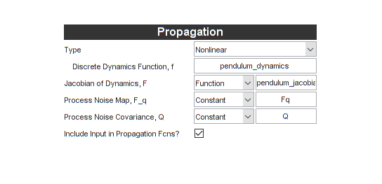
Let's tell it about our propagation function, propagation Jacobian function, and process noise covariance matrix.

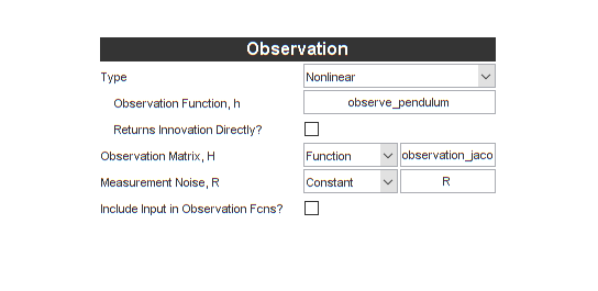
Let's do the same for the observation function, observation Jacobian, and measurement noise covariance matrix.

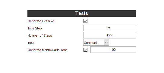
That was pretty quick, and we're almost ready to build the filter. However, we'd like *kf to automatically build a simulation and Monte-Carlo test for us, so we'll add options for those.

We'll tell *kf to use the time step we defined above, that we want 125 time steps in the simulation (resulting in a 5 second simulation), and that we want 100 runs in the Monte-Carlo test.

We're ready. Let's click the Generate Code button.

By default, all of the generated files will open in the editor. The four files it generates are:

An initialization function, pendulum_filter_init.m, which sets the initial conditions and constants,
A filter “step” function, pendulum_filter_step.m, which runs one time step of the filter,
An example simulation, pendulum_filter_example.m, which uses the propagation and observation functions along with process and measurement noise to build a true state and noisy observations over time and feeds these to the filter,
And a Monte-Carlo test, pendulum_filter_mc.m, which runs the above simulation 100 times and shows some statistics.

Let's take a look at the step function, which propagates the filter forward in time to a current measurement and performs the Kalman correction.

type pendulum_filter_step;

 
function [x, P] = pendulum_filter_step(t_km1, t_k, x, P, u_km1, z_k, constants)
 
% pendulum_filter_step
% 
% Inputs: 
% 
% t_km1         Time at sample k-1
% t_k           Time at sample k
% x             Estimated state at k-1 (prior)
% P             Estimate covariance at k-1 (prior)
% u_km1         Input vector at sample k-1
% z_k           Measurement at k
% constants     Constants struct from initialization function
% 
% Outputs: 
% 
% x             Estimated state at sample k
% P             Estimate error covariance at sample k
% 
% Generated with *kf v1.0.3
 
    %#codegen
 
    % Tell MATLAB Coder how to name the constants struct.
    coder.cstructname(constants, 'pendulum_filter_constants');
 
    % See if we need to propagate.
    if t_k > t_km1
 
        % Create the Jacobian of the propagation function wrt the state.
        F_km1 = pendulum_jacobian(t_km1, t_k, x, u_km1);
 
        % Linearly propagate the covariance.
        P = F_km1 * P * F_km1.' + constants.Q_eff;
 
        % Propagate the state.
        x = pendulum_dynamics(t_km1, t_k, x, u_km1);
 
    end % propagation frame
 
    % Create the observation matrix.
    H_k = observation_jacobian(t_k, x);
 
    % Predict the measurement.
    z_hat_k = observe_pendulum(t_k, x);
 
    % Innovation vector at sample k
    y_k = z_k - z_hat_k;
 
    % State-measurement covariance at k
    P_xy_k = P * H_k.';
 
    % Innovation covariance matrix at k (local)
    P_yy_k = H_k * P_xy_k + constants.R_k;
 
    % Safely calculate the Kalman gain.
    K = smrdivide(P_xy_k, P_yy_k);
 
    % Update the state estimate.
    x = x + K * y_k;
 
    % Build the matrix used for Joseph form covariance correction.
    A = -K * H_k;
    A = addeye(A);
 
    % Update the estimate covariance (Joseph form).
    P = A * P * A.';
    P = P + K * constants.R_k * K.';
 
end % pendulum_filter_step

Note all of the documentation and the clarity of the code. Of course, it's very generic since we haven't yet dug into the features of *kf, but this is just the intro. (To really get into the details, see the jaguar tutorial.)

We can now run the simulation to see how the filter performs.

pendulum_filter_example();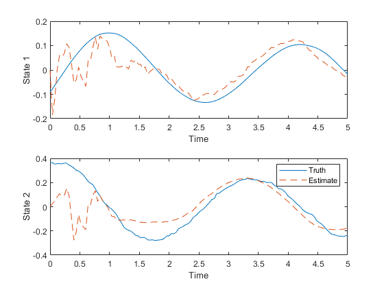

It looks like the estimated state (dashed line) has some trouble tracking the true state (solid line) right at the beginning, due to the large initial uncertainty and the nonlinearities, but then converges on the true state.

Is this good or bad? Let's run all 100 simulations in the Monte-Carlo test and take a look at the statistics.

pendulum_filter_mc();

NEES: Percent of data in theoretical 95.0% bounds: 75.4%
NMEE: Percent of data in theoretical 95.0% bounds: 94.8%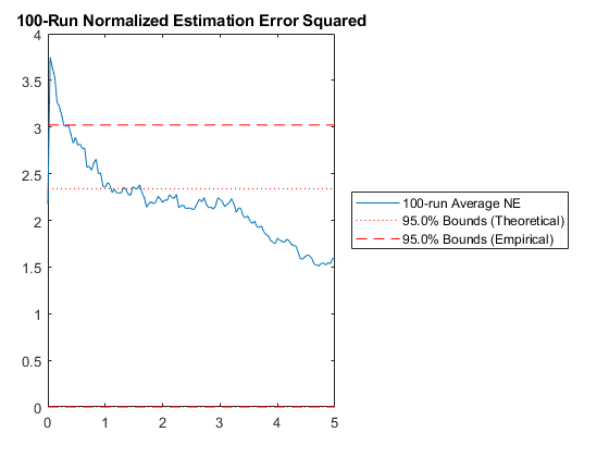

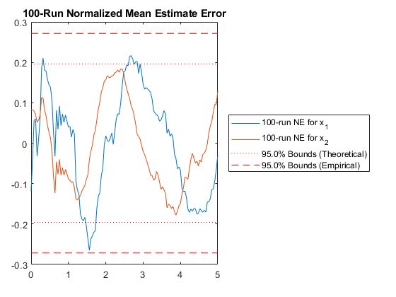
This shows us some aggregated statistics of all 100 runs. The two plots it generates show us how many of the estimation errors lie within the 95% confidence bounds predicted by the covariance matrices over time. Due to the nonlinearities, the filter is a little optimistic; that is, more than 5% of the errors are outside of the theoretical 95% bound created from the covariance matrix. This means that the covariance matrix doesn't capture the real distribution very well, which can lead to some problems.

There are a number of ways we might fix this. We might change the Jacobian calculation, use a smaller time step, or add consider covariance, but we'll opt to instead use an iterated extended Kalman filter. This type of filter helps the Kalman correction portion better capture the nonlinearities of the filter (see the documentation for more detail on this). Trying this is very easy with *kf, we'll just make one change in the options.

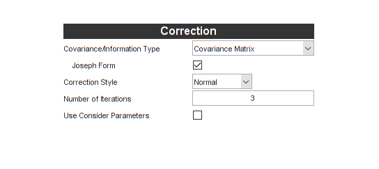
Iterated Extended Kalman Filter

All we need to do make this an iterated extended Kalman filter (IEKF) is tell *kf how many iterations we want. A single iteration is just a normal extended Kalman filter, so we'll need to use two or more to iterate. Let's try three iterations — two more than normal.

Let's click Generate Code to make the new filter, initialization function, simulation, and Monte-Carlo test.

We now have a new step function. It looks a little different to accomodate the iteration. Note how some calculations are outside of the iteration loop to save runtime while only the relevant calculations are inside of the loop. Also note that the filter “knows” to save the propagated variables (the _kkm1 forms), which weren't necessary before.

type pendulum_filter_step;

 
function [x, P] = pendulum_filter_step(t_km1, t_k, x, P, u_km1, z_k, constants)
 
% pendulum_filter_step
% 
% Inputs: 
% 
% t_km1         Time at sample k-1
% t_k           Time at sample k
% x             Estimated state at k-1 (prior)
% P             Estimate covariance at k-1 (prior)
% u_km1         Input vector at sample k-1
% z_k           Measurement at k
% constants     Constants struct from initialization function
% 
% Outputs: 
% 
% x             Estimated state at sample k
% P             Estimate error covariance at sample k
% 
% Generated with *kf v1.0.3
 
    %#codegen
 
    % Tell MATLAB Coder how to name the constants struct.
    coder.cstructname(constants, 'pendulum_filter_constants');
 
    % See if we need to propagate.
    if t_k > t_km1
 
        % Create the Jacobian of the propagation function wrt the state.
        F_km1 = pendulum_jacobian(t_km1, t_k, x, u_km1);
 
        % Linearly propagate the covariance.
        P_kkm1 = F_km1 * P * F_km1.' + constants.Q_eff;
 
        % Propagate the state.
        x_kkm1 = pendulum_dynamics(t_km1, t_k, x, u_km1);
 
    % Otherwise, the inputs have already been propagated.
    else
 
        % Explicitly copy the state.
        x_kkm1 = x;
 
        % Explicitly copy the covariance.
        P_kkm1 = P;
 
    end % propagation frame
 
    % Predict the measurement.
    z_hat_k = observe_pendulum(t_k, x_kkm1);
 
    % Innovation vector at sample k
    y_k = z_k - z_hat_k;
 
    % State estimate used for Jacobians for this iteration
    x = x_kkm1;
 
    % Iterate on the Kalman gain.
    for ii = 1:3
 
        % Create the observation matrix.
        H_k = observation_jacobian(t_k, x);
 
        % State-measurement covariance at k
        P_xy_k = P_kkm1 * H_k.';
 
        % Innovation covariance matrix at k (local)
        P_yy_k = H_k * P_xy_k + constants.R_k;
 
        % Safely calculate the Kalman gain.
        K = smrdivide(P_xy_k, P_yy_k);
 
        % Update the state estimate.
        x = x_kkm1 + K * y_k;
 
    end % iteration frame
 
    % Build the matrix used for Joseph form covariance correction.
    A = -K * H_k;
    A = addeye(A);
 
    % Update the estimate covariance (Joseph form).
    P = A * P_kkm1 * A.';
    P = P + K * constants.R_k * K.';
 
end % pendulum_filter_step

Let's go straight to Monte-Carlo testing the new filter to see if it has improved.

pendulum_filter_mc();

NEES: Percent of data in theoretical 95.0% bounds: 91.3%
NMEE: Percent of data in theoretical 95.0% bounds: 94.8%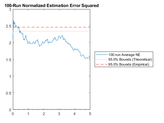

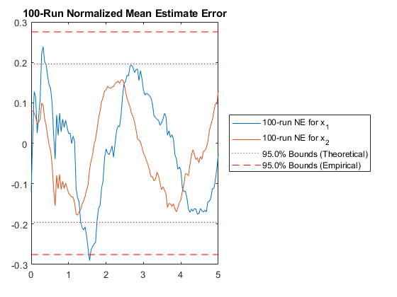
The statistics are better. That's a good start. We could now continue to make modifications, try new options, increase the number of runs in the Monte-Carlo test, and really make sure we're getting things right, but for now, we'll let the intro end here.

Next Steps

To examine the inputs to the *kf engine more deeply, see the jaguar tutorial.

To see how to use functions in *kf without the need of generating code, see the Eustace tutorial.

To read about the nomenclature used in *kf, about filter types, and about a good workflow for filter design, see the filter concepts page.

When you're ready, you can also try a homework problem to design a filter from scratch.

Our Problem
Extended Kalman Filter
Iterated Extended Kalman Filter
Next Steps

Docs