normerr

Returns the normalized error squared for signals in x with covariance C. For multiple runs, returns the n-run average normalized error squared. Returns also the fraction of points within the 100% * p probability bounds based on the number of runs. This can be used to determine if errors in x correspond appropriately to the covariance.

[err, f, b, errs] = normerr(x, C)
[err, f, b, errs] = normerr(x, C, p)
[err, f, b, errs] = normerr(x, C, p, type)
[err, f, b, errs] = normerr(x, C, p, type, (etc.))

Inputs

x	Residuals. For estimation error, `x - x_hat`. For measurement error, `z - z_hat`. Dimensions are `nx-ns-nr` (number of states, number of samples, and number of runs).
C	Covariance stored as `nx-nx-ns-nr` matrix. Alternately, for constant covariance across all runs and time stamps, just `nx-by-nx`.
p	Probability region (0 to 1) to examine. E.g., to compare the normalized residuals with a 95% probability region, use 0.95. Default is 0.95.
type	For type 1, the error `x.' * C^-1 * x` is used, giving a single normalized error magnitude for that sample. For type 2, the error `x ./ sqrt(diag(C))` is used, giving an error per state, normalized by each state's standard deviation. Default is 1.
(etc.)	Option-value pairs: `'OneSided' - True to use a one-sided distribution test (only used for type 1) 'Plot' - True to plot results 'Xdata' - Data to use for x values when plotting`

Outputs

err	N-run average normalized error (1-by-`ns`)
f	Fraction of points in `err` that are within the probability bounds
b	Probability bounds stored as `[low bound, high bound]`
errs	Matrix containing normalized error for each run individually (1-by-`ns`-by-`nr`), useful for finding which runs have excessive error

Example

Generate a large number of runs and samples per run of a 3-dimensional state with a different covariance matrix everywhere. See that the theoretical bounds and the empirical bounds determined by normerr match well.

% Define the sizes and preallocate space for the errors and covariance
% matrices.
nx = 3;                          % 3 states
nr = 25;                         % 25 runs
ns = 1000;                       % 1000 samples each
x  = zeros(nx, ns, nr);          % A place for all the residual data
C  = zeros(nx, nx, ns, nr);      % A place for each covariance matrix
 
% For each sample of each run, generate a random positive-definite
% covariance matrix and make a random draw from it.
for r = 1:nr
    for s = 1:ns
        C(:, :, s, r) = randcov(nx);
        x(:, s, r)    = mnddraw(C(:, :, s, r), 1);
    end
end

Examine what fraction of the data lay within the 90% confidence bounds (should be close to 0.90).

% For type 1 -- total state error
figure(1);
subplot(2, 1, 1);
[err1, f1] = normerr(x, C, 0.90, 1, 'Plot', true);
 
% For type 2 -- individual state error
subplot(2, 1, 2);
[err2, f2] = normerr(x, C, 0.90, 2, 'Plot', true);

Percent of data in theoretical 90.0% bounds: 88.1%
Percent of data in theoretical 90.0% bounds: 89.6%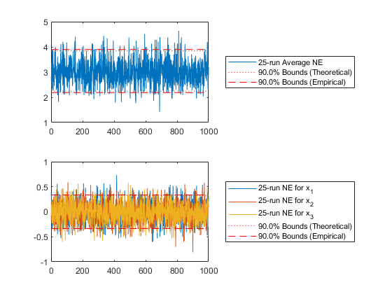

Docs

normerr

Inputs

Outputs

Example

See Also

Table of Contents