Counting Jaguars: *kf Engine Tutorial

This is the entry-level tutorial for the *kf engine. We'll look at building a simple filter to solve a generic problem, and then we'll begin to see what options are available to increase performance and decrease runtime.

If you have *kf installed, you can follow along with this tutorial:

skfexample('jaguars');

This will copy the example files into your local directory.

Problem Statement

Jaguars are very difficult to see in the wild. You could spend a lifetime romping through the jungle and never see one. It's hard to know how many live in the wild when you can't find them in the first place. Deer, however, are very easy to see in the wild, and jaguars prey on deer.

For the sake of an example, let's suppose we want to estimate the number of jaguars in a small, Central American country. We can't find them (without the use of harmful traps), so we'll try to figure out the numbers of jaguars by counting the deer and observing changes over time. To count the deer, we'll pick a few representative areas, count all the deer in those areas, and extrapolate a nation-wide total number of deer. That won't give us a perfect count of the number of deer, but it will give us something.

Next, we'll assume that the population of jaguars and deer are related. If there were one jaguar per deer, the deer population would likely decline rapidly. If there were only a hundred or so jaguars in the whole country, the deer population might increase due to lack of predation. This relationship is formalized in a simple mathematical model called the predator-prey model or Lotka-Volterra equation: $$\frac{dx_d}{dt} = a x_d - b x_d x_j$$ $$\frac{dx_j}{dt} = d x_d x_j - g x_j$$

where $x_d$ is the number of deer and $x_j$ is the number of jaguars (and the rest are constants). We'll use this model along with a series of different filters to determine the most likely population of jaguars. (This is of course not how real life science is carried out; this is just an extremely simple model that anyone can follow.)

Here's an example of the equations over 20 years with some arbitrary constants, where we're using a vector, $x$, of the two populations: $$x = \left[x_d, x_j\right]^T$$

% Choose arbitrary constants for the Lotka-Volterra equations.
a = 1.01;
b = 5e-4;
d = 1e-6;
g = 2;
 
% Simulate using MATLAB's built-in ode45.
ode = @(~, x) [a * x(1) - b * x(1) * x(2); ...
               d * x(1) * x(2) - g * x(2)];
[t, x] = ode45(ode, [0 20], [1e6; 1e3]);
 
% Plot the results.
figure(1);
subplot(2, 1, 1);
plot(t, x(:, 1));
ylabel('Deer');
subplot(2, 1, 2);
plot(t, x(:, 2));
ylabel('Jaguars');
xlabel('Time (years)');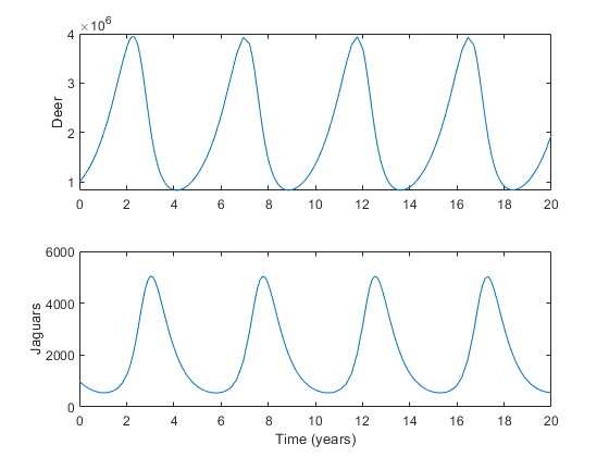

Detailed Problem Definition

To get started, just to keep things easy, we're going to assume we know $a$, $b$, $c$, and $d$ as constants in the jaguar-deer relationship, perhaps from studies in some other country. (We'll relax this later.)

To build an estimator with *kf, we're going to need to start with a description of our problem, and then we'll use *kf to build the estimator around this. For starters, we'll need:

A function to describe the propagation of the populations
A function to determine the expected number of deer (easy)
The noise in the measurement of the number of deer
The noise in the model (the magnitude of random population changes)

For the propagation function, we can simply use what we have above. We'll put it in a function called jaguar_dynamics.m which propagates the vector of populations, x_km1, which corresponds to the time at sample k-1 (t_km1) to x_k, corresponding to the time at sample k (t_k).

type jaguar_dynamics.m;

 
function x_k = jaguar_dynamics(t_km1, t_k, x_km1)
 
% jaguar_dynamics
%
% This function propagates the jaguar-deer state from sample k-1 to sample
% k.
%
% Inputs:
%
% t_km1  Time at sample k-1
% t_k    Time at sample k
% x_km1  State at sample k-1, consisting of populations of [deer; jaguars]
%
% Outputs:
%
% x_k    State updated to sample k
 
    % Make sure no population is less than 0 due to the noise.
    x_km1 = max(x_km1, 0);
    
    % Time step [years]
    dt = t_k - t_km1;
    
    % Propagate with a 4th-order Runge Kutta method.
    k1 = ode(x_km1);
    k2 = ode(x_km1 + 0.5 * dt * k1);
    k3 = ode(x_km1 + 0.5 * dt * k2);
    k4 = ode(x_km1 +       dt * k3);
    x_k = x_km1 + dt/6 * (k1 + 2*k2 + 2*k3 + k4);
 
end % jaguar_dynamics
 
% Continuous-time propagation function
function x_dot = ode(x)
 
    % We're assuming we know these constants:
    a = 1.01;
    b = 5e-4;
    d = 1e-6;
    g = 2;
    
    % Lotka-Volterra equation
    x_dot = [a * x(1) - b * x(1) * x(2); ...
             d * x(1) * x(2) - g * x(2)];
               
end % ode

Of course, the population also changes randomly too. We'll suppose that every three months, random effects change both populations. The deer change with a standard deviation of 50,000, while the jaguars change with a standard deviation of 20. (We will assume these random changes are appliedly discretely every time step in order to keep the math easy for now.)

% Standard deviation of random fluxation of deer and jaguars over 3 months.
sigma_deer    = 50000;
sigma_jaguars = 20;

Expressing the population noise as a covariance matrix, $Q$, we have:

Q = [sigma_deer^2, 0; ...
     0,            sigma_jaguars^2];

The standard deviations squared (the variance) goes on the diagonal, and the off-diagonal terms are 0 as there is no covariance between the "deer noise" and the "jaguar noise" for our example.

Later on, we can make this dynamic; the noise will vary with the size of the populations.

Now we need a measurement function, which will determine the number of deer we expect to "count", given the current populations, x_k. Of course, this is trivial. If we think our deer counting method has zero mean error, then if there x_d deer, we expect to count x_d. That means this is a short function.

type observe_deer.m;

 
function deer = observe_deer(t_k, x_k) %#ok
 
% observe_deer
%
% This function returns the expected observation of the number of deer 
% given the state. Of course, this is just the first element of the state,
% making this a pretty easy function.
 
    % The number of deer at t_k is just the first part of the state.
    deer = x_k(1);
 
end % observe_deer

Let's also define our measurement noise — how wrong our deer counts probably are (say, a standard deviation of 250,000 deer):

% Standard deviation and variation of the total deer count
sigma_deer = 250000;
R          = sigma_deer^2;

We've now described our problem. This is the part *kf couldn't possibly know about. But the rest — coding the actual filter, generating a simulation to exercise the filter, and even generating a Monte-Carlo test — are all things that *kf can do for us.

Building the Unscented Filter

We are now ready to begin building the filter in *kf. Let's start up the graphical user interface (GUI) to tell the *kf engine about our predator-prey estimation problem.

gui = skfengine();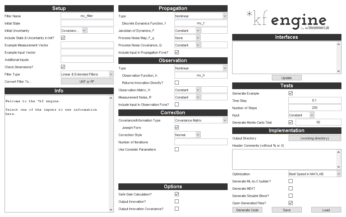

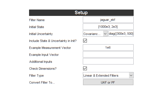
That looks like a lot of stuff. Fortunately, we need to fill in very little of it to get started. We can go back and add detail and improve the filter later.

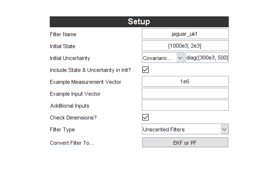
Let's get started with a few options:

The filter name (we'll call it jaguar_ukf)
The initial estimate for the populations, (1,000,000 deer, 2000 jaguars)
The initial covariance of the estimate (for our case, large initial uncertainty in the populations: 300,000 deer and 500 jaguars)

Let's also select "Unscented Filters". These are easier to start with than extended Kalman filters. They also generally have at least slight better performance on nonlinear problems.

Here's what we have:

Note that the help text changes when we enter something. Having just selected the Unscented Filters options, here's part of what it shows:

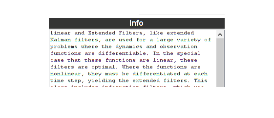
Right-clicking on the text, like "Filter Name", also shows the corresponding help.

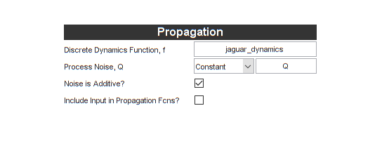
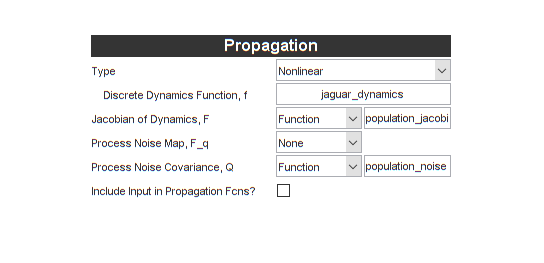
Let's enter the propagation function and process noise (we can just use the name of our function above, jaguar_dynamics and Q from the workspace). We'll also say that the noise is additive (it just adds on at the end of the update; it's not an input into the propagation function, which unscented filters allow). We don't use an "input" vector, so we can uncheck that box too.

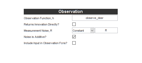
Now for the observation function and additive measurement noise. We'll use observe_deer and R from above.

That's it! We're ready to build a simple first-pass unscented Kalman filter (UKF)! Let's click on the "Update" button under "Interfaces". This will show the interface to all of our functions that the filter will call, and it also shows how we can call all of the functions that it generates. Let's make sure it plans to call jaguar_dynamics and observe_deer as we intend.

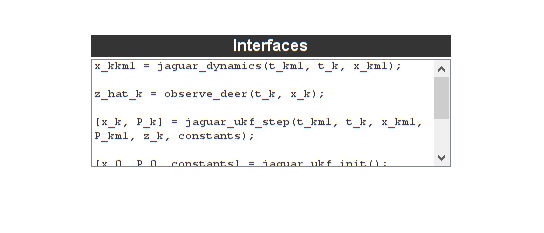
Yes, that matches our interfaces. (The filter generator will always expect to pass in the last time, current time, last estimate, current measurement, etc.).

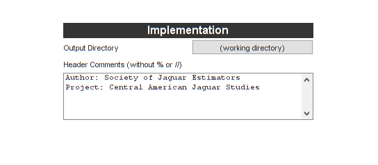
Let's add a header comment for the code we're going to generate, under "Implementation".

Let's also tell it to generate some tests while we'll at it. We'll let the time step be 0.25, so this will correspond to a "deer measurement" every quarter of a year (for our problem, $t$ has units of years). Then we'll simulate for 80 steps, or 80*0.25 = 20 years.

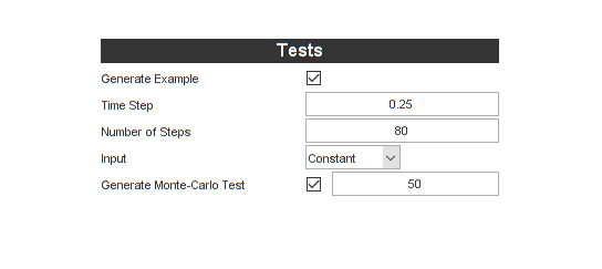
Now let's click "Generate Code".

Exercising the Filter

It finished. Let's see how well the filter does. The usual way to do this is to create a simulator, propagate a "truth" model, generate noisy measurements from the truth model, and feed those noisy measurements into the filter function over time. Fortunately, *kf does this for us, using the propagation function and noise for truth and the measurement function and noise for the measurements. This both shows us how to integrate the generated filter function and serves as a quick simulation.

Let's run it:

% Run the simulation.
[t, x, x_hat] = jaguar_ukf_example();
 
% Plot the results.
figure(1);
subplot(2, 1, 1);
plot(t, x(1, :), t, x_hat(1, :), '--');
ylabel('Deer');
legend('True', 'Estimated', 'Location', 'NorthEast');
subplot(2, 1, 2);
plot(t, x(2, :), t, x_hat(2, :), '--');
ylabel('Jaguars');
xlabel('Time (years)');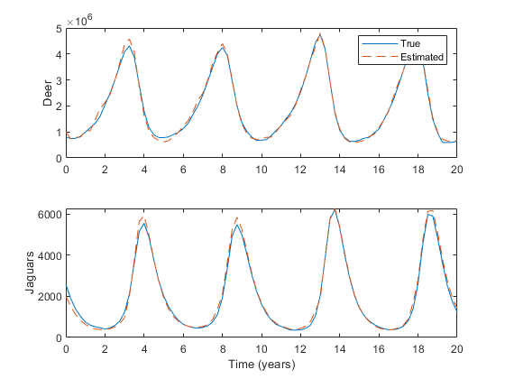

The simulation uses the initial estimate value we entered earlier, and generates an initial true state using the initial covariance matrix. It then propagates the true state using our propgation function and process noise, makes measurements using our observation function and observation noise, and calls the filter with the measurement in order to update the estimate over time. It does this with a lot of random draws, so every time we run it, it will be slightly different.

% Run the simulation again.
[t, x, x_hat] = jaguar_ukf_example();
 
% Plot the results.
figure(1);
subplot(2, 1, 1);
plot(t, x(1, :), t, x_hat(1, :), '--');
ylabel('Deer');
legend('True', 'Estimated', 'Location', 'NorthEast');
subplot(2, 1, 2);
plot(t, x(2, :), t, x_hat(2, :), '--');
ylabel('Jaguars');
xlabel('Time (years)');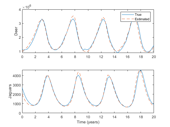

We can get a feel for how to integrate our filter into whatever project we're working on by looking at the example simulation:

type jaguar_ukf_example.m;

 
function [t, x_true, x_hat, P] = jaguar_ukf_example()
 
% jaguar_ukf_example
% 
% Example simulation for jaguar_ukf_step().
% 
% Inputs: 
% 
% 
% 
% Outputs: 
% 
% t             Time history of simulation
% x_true        History of true state
% x_hat         History of estimated state
% P             History of estimate covariance
% 
% Generated with *kf v1.0.3
 
    % Time step
    dt = 0.25;
 
    % Number of time steps
    nt = 80;
 
    % Create the time history.
    t = 0:dt:nt*dt;
 
    % Run the filter initialization.
    [x_hat_0, P_0, constants] = jaguar_ukf_init();
 
    % Dimension of the state
    nx = length(x_hat_0);
 
    % Create an initial true state.
    x_true_0 = x_hat_0 + sqrtpsdm(P_0) * randn(nx, 1);
 
    % Preallocate for the true state history.
    x_true = [x_true_0, zeros(nx, nt)];
 
    % Preallocate for the estimated state history.
    x_hat = [x_hat_0, zeros(nx, nt)];
 
    % Preallocate for the estimate covariance history.
    P = cat(3, P_0, zeros(nx, nx, nt));
 
    % Dimension of the process noise
    nq = size(constants.sqQ, 1);
 
    % Dimension of the measurement noise
    nr = size(constants.R_k, 1);
 
    % Matrix square-root of the measurement noise covariance
    sqR = sqrtpsdm(constants.R_k);
 
    % For each time step, simulate the true dynamics and run the filter.
    for k = 2:nt+1
 
        % Draw the process noise for this sample.
        q_km1 = constants.sqQ * randn(nq, 1);
 
        % Propagate the true state.
        x_true(:,k) = jaguar_dynamics(t(k-1), t(k), x_true(:,k-1)) + q_km1;
 
        % Draw the measurement noise for this sample.
        r_k = sqR * randn(nr, 1);
 
        % Create the noisy measurement.
        z_k = observe_deer(t(k), x_true(:,k)) + r_k;
 
        % Propagate and update the estimate with the new measurement.
        [x_hat(:,k), P(:,:,k)] = jaguar_ukf_step(t(k-1), t(k), x_hat(:,k-1), P(:,:,k-1), z_k, constants);
 
    end % main loop
 
    % If there are no outputs, plot it.
    if nargout == 0
        unique_figure('jaguar_ukf_example');
        for k = 1:nx
            subplot_geometry(nx, k);
            plot(t, x_true(k,:), t, x_hat(k,:), '--');
            xlabel('Time');
            ylabel(sprintf('State %d', k));
        end
        legend('Truth', 'Estimate');
    end
 
end % jaguar_ukf_example

There are two lines in here that show us how to incorporate the filter. The first sets up the initial estimate, initial covariance, and any constants used by the filter. We run this once, right at the beginning.

% Initialize the filter variables.
[x_hat_0, P_0, constants] = jaguar_ukf_init();

Next, there's the call to the function that performs the filtering for the current time step:

[x_hat(:,k), P(:,:,k)] = jaguar_ukf_step(t(k-1), t(k), ...
                             x_hat(:,k-1), P(:,:,k-1), z_k, constants);

This shows how to pass in the previous and current times, previous estimate and covariance, current measurement, and the constants (from initialization). The output is the updated state and covariance. All told, that's pretty easy.

(The generated filter will always have a name that's just (filter_name)_step.)

The Generated UKF

So we now know how to call the filter that we've generated. But what does it actually look like? This one is pretty long:

type jaguar_ukf_step;

 
function [x, P] = jaguar_ukf_step(t_km1, t_k, x, P, z_k, constants)
 
% jaguar_ukf_step
% 
% Author: Society of Jaguar Estimators
% Project: Central American Jaguar Studies
% 
% Inputs: 
% 
% t_km1         Time at sample k-1
% t_k           Time at sample k
% x             Estimated state at k-1 (prior)
% P             Estimate covariance at k-1 (prior)
% z_k           Measurement at k
% constants     Constants struct from initialization function
% 
% Outputs: 
% 
% x             Estimated state at sample k
% P             Estimate error covariance at sample k
% 
% Generated with *kf v1.0.3
 
    %#codegen
 
    % Tell MATLAB Coder how to name the constants struct.
    coder.cstructname(constants, 'jaguar_ukf_constants');
 
    % Dimension of the state
    nx = length(x);
 
    % Dimension of the measurement
    nz = length(z_k);
 
    % Dimension of the process noise
    nq = size(constants.sqQ, 1);
 
    % Start and stop indices of components of sigma points
    x_stop  = nx;
    q_start = nx;
    q_stop  = nx + nq;
 
    % Matrix square-roots
    sqP = sqrtpsdm(P); % Matrix square-root of the estimate covariance
 
    % Size of augmented system
    L = nx + nq;
 
    % Tuning parameter
    kappa = 3 - L;
 
    % Weights
    lambda = constants.alpha^2 * (L + kappa) - L;
    gamma  = sqrt(L + lambda);
    W_m_0  = lambda / (L + lambda);
    W_c_0  = W_m_0 + 1 - constants.alpha^2 + constants.beta;
    W_i    = 1/(2*(L + lambda));
 
    % Propagate the expected state.
    x_kkm1_1 = jaguar_dynamics(t_km1, t_k, x);
 
    % Observe the expected state.
    z_hat_kkm1_1 = observe_deer(t_k, x_kkm1_1);
 
    % Preallocation
    x_kkm1_sps = zeros(nx, 2*L);
    z_hat_kkm1_sps = zeros(nz, 2*L);
 
    % Begin the mean state prediction, taking advantage of 
    % the fact that the process noise is additive.
    x_kkm1 = (W_m_0 + 2 * nq * W_i) * x_kkm1_1;
 
    % Begin the mean observation prediction.
    z_hat_kkm1 = W_m_0 * z_hat_kkm1_1;
 
    % Loop over each sigma point.
    for sp = 1:L
 
        % Create the positively displaced sigma point.
        if sp <= x_stop
            x_km1_p = x + gamma * sqP(1:nx, sp);
        else
            x_km1_p = x;
        end
 
        % Create the process noise for the positive sigma point.
        if sp > q_start && sp <= q_stop
            q_km1 = gamma * constants.sqQ(:, sp-q_start);
        else
            q_km1 = zeros(nq, 1);
        end
 
        % Propagate the positive sigma point.
        if sp > q_start && sp <= q_stop
            x_kkm1_sps(:, sp) = x_kkm1_1 + q_km1;
        else
            x_kkm1_sps(:, sp) = jaguar_dynamics(t_km1, t_k, x_km1_p);
        end
 
        % Observe the positive sigma point.
        z_hat_kkm1_sps(:, sp) = observe_deer(t_k, x_kkm1_sps(:, sp));
 
        % Create the negatively displaced sigma point.
        if sp <= x_stop
            x_km1_n = x - gamma * sqP(1:nx, sp);
        else
            x_km1_n = x;
        end
 
        % Create the process noise for the negative sigma point.
        if sp > q_start && sp <= q_stop
            q_km1 = -q_km1;
        end
 
        % Propagate the negative sigma point.
        if sp > q_start && sp <= q_stop
            x_kkm1_sps(:, L+sp) = x_kkm1_1 + q_km1;
        else
            x_kkm1_sps(:, L+sp) = jaguar_dynamics(t_km1, t_k, x_km1_n);
        end
 
        % Observe the negative sigma point.
        z_hat_kkm1_sps(:, L+sp) = observe_deer(t_k, x_kkm1_sps(:, L+sp));
 
        % For maximum numerical stability, add on these two sigma
        % points to the mean prediction simultaneously. Their sum is
        % only non-zero for the first several terms.
        if sp <= nx
            x_kkm1 = x_kkm1 + W_i * (x_kkm1_sps(:, sp) + x_kkm1_sps(:, L+sp));
        end
 
        % For maximum numerical stability, add on these two sigma
        % points to the mean observation prediction simultaneously.
        z_hat_kkm1 = z_hat_kkm1 + W_i * (z_hat_kkm1_sps(:, sp) + z_hat_kkm1_sps(:, L+sp));
 
    end % sigma points
 
    % Remove the sample means from the sigma points.
    x_kkm1_1 = x_kkm1_1 - x_kkm1;
    z_hat_kkm1_1 = z_hat_kkm1_1 - z_hat_kkm1;
    x_kkm1_sps = bsxfun(@minus, x_kkm1_sps, x_kkm1);
    z_hat_kkm1_sps = bsxfun(@minus, z_hat_kkm1_sps, z_hat_kkm1);
 
    % State-measurement covariance at k
    P_xy_k = W_c_0 * (x_kkm1_1 * z_hat_kkm1_1.') + W_i * (x_kkm1_sps * z_hat_kkm1_sps.');
 
    % Innovation covariance matrix at k
    P_yy_k = W_c_0 * (z_hat_kkm1_1 * z_hat_kkm1_1.') + W_i * (z_hat_kkm1_sps * z_hat_kkm1_sps.') + constants.R_k;
 
    % Estimate covariance at k based on information from k-1 (prior)
    P = W_c_0 * (x_kkm1_1 * x_kkm1_1.') + W_i * (x_kkm1_sps * x_kkm1_sps.');
 
    % Kalman gain
    K = smrdivide(P_xy_k, P_yy_k);
 
    % Innovation vector at sample k
    y_k = z_k - z_hat_kkm1;
 
    % Estimated state at sample k
    x = x_kkm1 + K * y_k;
 
    % Estimate error covariance at sample k
    P = P - K * P_yy_k * K.';
 
end % jaguar_ukf_step

UKFs are not trivial! Note that this is not a generic function; it's tailored to our specific problem, including our assumptions that the process and measurement noise are "additive" (remember checking that box?).

If you're familiar with unscented Kalman filters, you'll notice it's also doing a few intelligent things. For instance, since the noise is additive, the filter can use fewer sigma points and few propagation function evaluations than otherwise. Further, since the process noise and measurement noise are constant, they are decomposed in the initialization function, which is called once to set up the filter, and not in the step function! Plus, it's doing so safely, using sqrtpsdm ("square-root of a positive, semi-definite matrix") and smrdivide ("safe matrix right divide") to gracefully handle the case that the a covariance matrix might have zero eigevalues due to numerical roundoff or some such thing.

sqP = sqrtpsdm(P); % Matrix square-root of the estimate covariance
...
K_k = smrdivide(P_xy_k, P_yy_k_i);

Also, there are many, many comments. This is serious code!

Monte-Carlo Testing

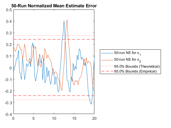
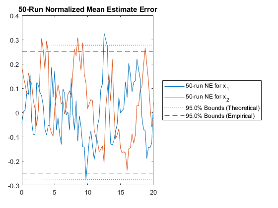
Running a single simulation or two is nice, but is always begs the question, "How much of the performance that I'm seeing is due to the initial draws? How will it perform in general?" This is where Monte-Carlo testing comes in. A Monte-Carlo (MC) test rather simply runs the example simulation numerous times (50 by default), each from a different starting point. It then examines the error between the simulated true state and the estimated state at each step of each run or a simulation. It considers these errors with their corresponding covariance to tell us if the covariance actually matches the errors it's seeing. That is, if the covariance indicates that a state estimate has a standard deviation of 1000 deer and 10 jaguars, then if we were to average the errors, we should see about an average error of 1000 deer and 10 jaguars. If the errors are greater, then the filter is optimistic — it thinks it's estimating better than it actually is. That's bad. It means the filter begins to ignore observations more than it should, instead favoring propagation to an unjustified degree.

(In order to compare the errors across multiple runs, which of course have different covariance matrices at each step, it doesn't actually compare the errors themselves. It first normalizes the errors by the covariance matrix in two different ways, and then works with average normalized error. This allows us to draw general conclusions from different data. Nice, yes?)

*kf generates a function to run a Monte-Carlo test for us, called, in this case, jaguar_ukf_mc. Let's run it and see if approximately 95% of our errors are inside the 95% confidence bound predicted by the covariance matrix.

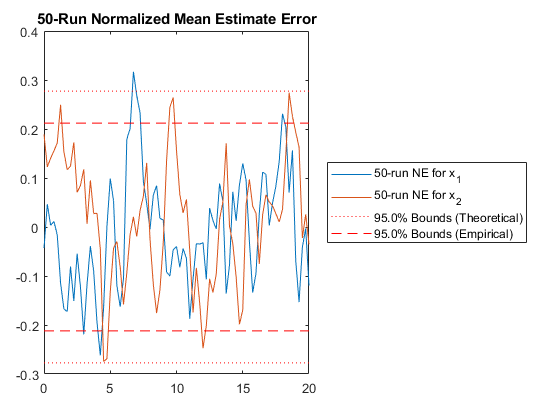
jaguar_ukf_mc();

NEES: Percent of data in theoretical 95.0% bounds: 95.1%
NMEE: Percent of data in theoretical 95.0% bounds: 96.3%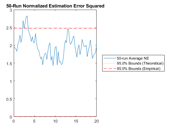

It looks like our filter is consistent, which means our filter is working well according to the assumptions we've made, such as that we've modeled the problem well. (There's more about all of these tests in the manual. See "Testing".)

Compared to the previous functions, the MC function is pretty short:

type jaguar_ukf_mc.m;

 
function [t, x_true, x_hat, P, errs] = jaguar_ukf_mc()
 
% jaguar_ukf_mc
% 
% Monte-Carlo runs for jaguar_ukf_example().
% 
% Inputs: 
% 
% 
% 
% Outputs: 
% 
% t             Time history of simulation
% x_true        History of true state
% x_hat         History of estimated state
% P             History of estimate covariance
% errs          Estimation errors
% 
% Generated with *kf v1.0.3
 
    % Dimensions
    x_0 = [1000000;2000]; % Initial state estimate
    ns = 50; % Number of simulations
    nt = 80; % Number of time steps
    nx = length(x_0); % Dimension of the state
 
    % Preallocation
    x_true = zeros(nx, nt+1, ns); % Preallocation for the true state history
    x_hat = zeros(nx, nt+1, ns); % Preallocation for the estimate history
    P = zeros(nx, nx, nt+1, ns); % Preallocation for the covariance history
 
    % For each run...
    for r = 1:ns
 
        % Set the random number generator seed for repeatability.
        rng(r);
 
        % Run the simulation.
        [t, x_true(:,:,r), x_hat(:,:,r), P(:,:,:,r)] = jaguar_ukf_example();
 
    end % each run
 
    % Estimation errors
    errs = x_true - x_hat;
 
    % NEES
    unique_figure('jaguar_ukf_NEES');
    clf();
    fprintf('NEES: ');
    normerr(errs, P, 0.95, 1, 'OneSided', true, 'XData', t);
    title('50-Run Normalized Estimation Error Squared');
 
    % NMEE
    unique_figure('jaguar_ukf_NMEE');
    clf();
    fprintf('NMEE: ');
    normerr(errs, P, 0.95, 2, 'XData', t);
    title('50-Run Normalized Mean Estimate Error');
 
end % jaguar_ukf_mc

Wrap-Up of the First UKF

We've generated a working filter, a simulator, and a Monte-Carlo wrapper to tell us how the filter is working. Notice what tiny fraction of the total code base was written by hand. Further, since the generated code is just regular (readable) code, we could start a more detailed simulator from the generated simulator. For instance, could see what would happen if the filter's initial covariance were different from the true covariance by adding a line like:

P_true_0 = [...];

to the example file and using that to create the initial true state.

x_true_0 = x_hat_0 + sqrtpsdm(P_true_0) * randn(nx, 1);

Our filter would certainly be much less consistent in the Monte-Carlo tests, but would it track at all or fall apart? This is just an example of a starting point for modifying the generated example file.

Note that if you generate a new filter, it will overwrite jaguar_ukf_example, so we should rename the file once we start changing it.

Another UKF

Up to this point, we've said that the deer and jaguar populations experience random, uncorrelated fluctuations every three months. Let's change this a bit and say that the random population changes are due to a single random variable representing deforestation. Positive deforestation means that forest is disappearing, and and some percentage of jaguars along with it. Negative deforestation means that it's growing back.

Let's call the deforestation $q$ and give it a variance (or 1-by-1 covariance matrix), $Q$, of 1 unit of deforestation. Then, we'll say that the jaguar population decreases discretely by $0.02 x_j q$, or 2% of its population per unit of deforestation. Similarly, the deer can decrease by $0.005 x_d q$ (deer are pretty adaptable). This means two things: first, our propagation function need to change to take in $q$ at each time step; second, our process noise is no longer additive, but an integral part of the nonlinear propagation function.

So let's rewrite the propagation function to take this into account, calling it jaguar_dynamics_2. Note the q_km1 input.

type jaguar_dynamics_2;

 
function x_k = jaguar_dynamics_2(t_km1, t_k, x_km1, q_km1)
 
% jaguar_dynamics_2
%
% This function propagates the jaguar-deer state from sample k-1 to sample
% k when there is an additional detrimental effect on the populations due
% to deforestation.
%
% Inputs:
%
% t_km1  Time at sample k-1
% t_k    Time at sample k
% x_km1  State at sample k-1, consisting of populations of [deer; jaguars]
%
% Outputs:
%
% x_k    State updated to sample k
 
    % Include the effects of deforestation.
    x_km1(1) = x_km1(1) - 0.02 * x_km1(1) * q_km1;
    x_km1(2) = x_km1(2) - 0.05  * x_km1(2) * q_km1;
 
    % Make sure no population is less than 0 due to the noise.
    x_km1 = max(x_km1, 0);
    
    % Time step [years]
    dt = t_k - t_km1;
    
    % Propagate with a 4th-order Runge Kutta method.
    k1 = ode(x_km1);
    k2 = ode(x_km1 + 0.5 * dt * k1);
    k3 = ode(x_km1 + 0.5 * dt * k2);
    k4 = ode(x_km1 +       dt * k3);
    x_k = x_km1 + dt/6 * (k1 + 2*k2 + 2*k3 + k4);
 
end % jaguar_dynamics_2
 
% Continuous-time propagation function
function x_dot = ode(x)
 
    % We're assuming we know these constants:
    a = 1.01;
    b = 5e-4;
    d = 1e-6;
    g = 2;
    
    % Lotka-Volterra equation
    x_dot = [a * x(1) - b * x(1) * x(2); ...
             d * x(1) * x(2) - g * x(2)];
               
end % ode

Let's set the variance of the deforestation, $Q$, to be 1 unit.

Q = 1;

Similarly, let's make the measurement noise be a fraction of the current population. If $r$ is the percent error and its standard deviation is 10% then we have:

R = 0.1^2;

and the new observation function:

type observe_deer_2;

 
function deer = observe_deer_2(t_k, x_k, r_k) %#ok
 
% observe_deer_2
% 
% This function returns the measured number of deer when the measurement
% error depends on the number of deer (the error is a percentage of the
% current population).
 
    % The number of deer at t_k is just the first part of the state.
    deer = x_k(1) + r_k * x_k(1);
 
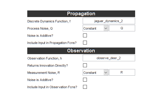
end % observe_deer_2

Let's put these values in the GUI. To summarize, we:

Changed the propagation function name
Unchecked the "Noise is Additive?" box for the process noise
Changed the measurement function name
Unchecked the "Noise is Additive?" box for the measurement noise

We can also change the name of the filter to jaguar_ukf_2 so that we don't overwrite our old filter.

Let's do one more thing. If you ran the Monte-Carlo test for the last filter, you surely noticed that it took a while to run. The best way to get better speed is to make sure the propagation and observation functions are coded well, and to select good options for the filter. However, if MATLAB Coder is installed, we can also get a great speed boost by compiling our filter's step function to a MEX file. Let's check the Generate MEX box. The MEX file will be built automatically, and the simulation will use the MEX instead of the MATLAB function. This will go much faster. (Don't check this box if you don't have MATLAB Coder.)

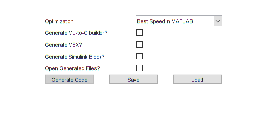
We can click "Generate Code", everything should work, and we can now run our new simulation.

% Run the new simulation.
[t, x, x_hat] = jaguar_ukf_2_example();
 
% Plot the results.
figure(1);
subplot(2, 1, 1);
plot(t, x(1, :), t, x_hat(1, :), '--');
ylabel('Deer');
legend('True', 'Estimated', 'Location', 'NorthEast');
subplot(2, 1, 2);
plot(t, x(2, :), t, x_hat(2, :), '--');
ylabel('Jaguars');
xlabel('Time (years)');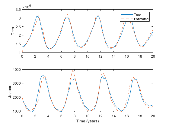

Looks good. Let's try the Monte-Carlo tests.

jaguar_ukf_2_mc();

NEES: Percent of data in theoretical 95.0% bounds: 96.3%
NMEE: Percent of data in theoretical 95.0% bounds: 99.4%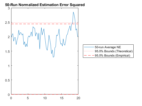

Excellent.

This is as far as this tutorial goes for unscented Kalman filters. We created a total of four very easy functions by hand and set only four variables in the workspace, and we used these to generate two custom filters, the corresponding initilization functions, simulations, Monte-Carlo tests, and a compiled MEX file for the final filter. We're in pretty good shape to play with the system at this point to see what else we can do, but that's an exercise for later. Let's now look at the namesake of *kf: Kalman filters.

Linear & Extended Kalman Filters

Linear and extended Kalman filters are much faster than UKFs (there is much in the literature about their being "of the same order", but Kalman filters are often several times faster and, under certain conditions, can require only a few percent of the runtime with about half of the memory usage). Kalman filters are like C/C++. They take a little more work, but they're much faster than any alternative with similar estimation power.

(Here, we're grouping information filters with Kalman filters; information filters can be faster when the number of observations is larger than the number of states.)

The flip side of speed, however, is performance. For highly nonlinear problems, unscented Kalman filters often estimate with lower error.

Let's see how we can build an extended Kalman filter for our jaguar example. First, let's rename the filter and select Linear and Extended Filters.

Now, under Propagation, we need a propagation function. A propagation function for a UKF with additive noise has the same interface as for an EKF, so we can reuse the same function from our first filter (jaguar_dynamics). Also, we can again uncheck the box for including an input vector.

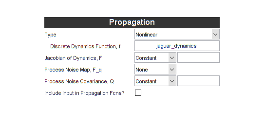
It's also asking for two more things, the matrices $F$ and $Q$. These will both be a little different than for the UKF. This brings us to Jacobians.

Jacobians and Noise Covariance

Caution: building the Jacobians and noise matrices is always the difficult part of building an extended Kalman filter. The fact that UKFs don't need Jacobians is one of the many features that make them attractive. However, for real-world applications, we very, very often need linear filters for performance. Now's a good time for a break.

Whereas the unscented Kalman filter uses several different propgations of related sigma points to determine the uncertainty of the state after propagation, linear filters use matrices to perform these updates on the covariance (simple multiplication and hence "linear"). These matrices are the Jacobians of the propagation and observation functions. The Jacobian is the partial difference of the output of a function with respect to its inputs. For instance, if our continuous-time propagation function is called $f$ and our state is called $x$, such that: $$x = \begin{bmatrix}x_d \\ x_j\end{bmatrix}$$ $$\dot{x} = f(x)$$

then the continuous-time Jacobian, $A$, about some reference state, $x_0$ is: $$A_{r,c} = \left. \frac{\partial}{\partial x_c} f_r \right\rvert_{x_0}$$

or more compactly: $$A = \left. \frac{\partial}{\partial x} f \right\rvert_{x_0}$$

For our problem: $$A = \left. \begin{bmatrix} \frac{\partial}{\partial x_d} (a x_d - b x_d x_j) & \frac{\partial}{\partial x_j} (a x_d - b x_d x_j) \\ \frac{\partial}{\partial x_d} (d x_d x_j - g x_j) & \frac{\partial}{\partial x_j} (d x_d x_j - g x_j) \\ \end{bmatrix} \right\rvert_{x_0} $$ $$A = \left. \begin{bmatrix} a - b x_j & - b x_d \\ d x_j & d x_d - g \\ \end{bmatrix} \right\rvert_{x_0} $$

Note that this is the Jacobian of the continuous-time system. For the extended Kalman filter, we'll need the Jacobian of the discrete-time system. We can convert this one of two ways. We can create a discrete version of the Lotka-Volterra equations ($f$), or we can simply discretize $A$ as a usually-acceptable approximation. Let the discrete-time Jacobian be $F$. $$F = e^{A \Delta t}$$

where this is clearly a matrix exponential (expm in MATLAB) and $\Delta t$ is the time step (we've been using 0.25 for a quarter of a year). There are different ways to discretize a continuous-time system such as this; a matrix exponential is accurate, but computationally expensive.

Let's create a function for this:

type population_jacobian.m;

 
function F = population_jacobian(t_km1, t_k, x)
 
% population_jacobian
%
% This function calculate the Jacobian of the discrete-time dynamics of the
% deer-jaguar system by first calculating the Jacobian of the
% continuous-time Lotka-Volterra equation and then discretizing.
 
    % We're assuming we know these constants:
    a = 1.01;
    b = 5e-4;
    d = 1e-6;
    g = 2;
 
    % Continuous-time Jacobian of the Lotka-Volterra equation
    A  = [a - b*x(2), -b*x(1); ...
          d*x(2),     d*x(1) - g];
      
    % Time step [years]
    dt = t_k - t_km1;
    
    % Discretize to closely approximate the Jacobian of the discrete-time 
    % system
    F  = expm(A * dt);
 
end % population_jacobian

Moving on to the process noise, let's recall that our process noise is now a nonlinear function that includes the current population and the current amount of deforestation, so the effect of the noise on deer and jaguars respectively is: $-0.02 x_d q$ and $-0.05 x_j q$. Representating the the full state $x = \left[x_d, x_j\right]^T$, the effect of noise, $q_e$ is: $$q_e = \begin{bmatrix} 0.02 x_d \\ 0.05 x_j\end{bmatrix} q$$

Since the variance of $q$ is $Q$, the covariance of $q_e$, $Q_e$, is: $$Q_e = \begin{bmatrix} 0.02 x_d \\ 0.05 x_j\end{bmatrix} Q \begin{bmatrix} 0.02 x_d && 0.05 x_j\end{bmatrix}$$

(ignoring the uncertainty associated with the state).

Let's make a function to generate Q given the current state. This is actually easy:

type population_noise;

 
function Q_e = population_noise(t_km1, t_k, x_km1) %#ok
 
% population_noise
%
% This function calculates the effective covariance for sample k-1 of the
% random effects of deforestation. It assumes that the deforestation noise
% maps to deer and jaguar populations such that 1 "unit" of deforestation
% maps to a 2% population decline in deer and 5% in jaguars.
%
% See jaguars_tutorial.m for a discussion.
 
    % Deforestation variance
    Q = 1;
    
    % Map from deforestation (q) to effect on populations (dx = F_q * q)
    F_q = [0.02 * x_km1(1); ...
           0.05 * x_km1(2)];
    
    % Effective covariance
    Q_e = F_q * Q * F_q.';
 
end % population_noise

We now put these both into the interface:

Ok, in terms of the actual coding, that wasn't too bad. Let's move on the the observation function and measurement noise.

The observation function part is actually much easier. Since our observation function simply "selects" the deer population, there's a special form for this in *kf (it's reasonably common). For Type, we'll pick Subset, and then enter a 1, meaning that the observation is simply the first index of the state.

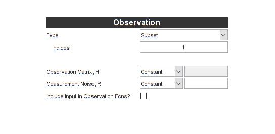
Note that the Jacobian is greyed out. It's unnecessary now. Using this "subset" type will actually make the filter run faster than using the Jacobian (which is [1 0]) directly.

We can now tackle $R$ just like we did for $Q$. The observation error that we were using had a standard deviation of 10% of the population size of the deer. $R$ was simply $0.1^2$. Let $r_e$ be the effect on the observation, with variance $R_e$. This is now given by: $$R_e = x_d R x_d$$

or, as a function:

type observation_noise;

 
function R_e = observation_noise(t_k, x_k) %#ok
 
% observation_noise
%
% Return the measurement noise covariance when it depends on the current
% population of deer.
 
    % Variance of error as percentage of the population
    R = 0.1^2;
    
    % Variance of population measurement
    R_e = x_k(1) * R * x_k(1);
 
end % observation_noise

Let's select Function and enter this in the GUI.

Building the Extended Kalman Filter

That was certainly more work than we put into the UKF, but now we're ready to build. However, before building, let's tell the filter to give us two more pieces of information we can use to evaluate performance: the innovation vector (difference between the measurement and the predicted observation) and its covariance.

Let's turn off the Generate MEX option (the filter is plenty fast as it is), and generate the new code.

Running the example:

% Run the new simulation.
[t, x, x_hat] = jaguar_ekf_example();
 
% Plot the results.
figure(1);
subplot(2, 1, 1);
plot(t, x(1, :), t, x_hat(1, :), '--');
ylabel('Deer');
legend('True', 'Estimated', 'Location', 'NorthEast');
subplot(2, 1, 2);
plot(t, x(2, :), t, x_hat(2, :), '--');
ylabel('Jaguars');
xlabel('Time (years)');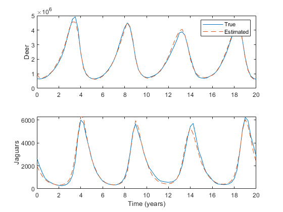

Looking at the code, we can see that this linear filter is substantially shorter than the unscented filters. Note the extra outputs for the innovation and innovation covariance.

type jaguar_ekf_step;

 
function [x, P, y_k, P_yy_k] = jaguar_ekf_step(t_km1, t_k, x, P, z_k)
 
% jaguar_ekf_step
% 
% Author: Society of Jaguar Estimators
% Project: Central American Jaguar Studies
% 
% Inputs: 
% 
% t_km1         Time at sample k-1
% t_k           Time at sample k
% x             Estimated state at k-1 (prior)
% P             Estimate covariance at k-1 (prior)
% z_k           Measurement at k
% 
% Outputs: 
% 
% x             Estimated state at sample k
% P             Estimate error covariance at sample k
% y_k           Innovation vector at sample k
% P_yy_k        Innovation covariance matrix at k
% 
% Generated with *kf v1.0.3
 
    %#codegen
 
    % Indices of the state that are directly observed
    z_ind = 1;
 
    % Dimension of the state
    nx = length(x);
 
    % See if we need to propagate.
    if t_k > t_km1
 
        % Create the Jacobian of the propagation function wrt the state.
        F_km1 = population_jacobian(t_km1, t_k, x);
 
        % Create the process noise covariance matrix.
        Q_km1 = population_noise(t_km1, t_k, x);
 
        % Linearly propagate the covariance.
        P = F_km1 * P * F_km1.' + Q_km1;
 
        % Propagate the state.
        x = jaguar_dynamics(t_km1, t_k, x);
 
    end % propagation frame
 
    % Create the measurement noise covariance.
    R_k = observation_noise(t_k, x);
 
    % Predict the measurement.
    z_hat_k = x(z_ind);
 
    % Innovation vector at sample k
    y_k = z_k - z_hat_k;
 
    % State-measurement covariance at k
    P_xy_k = P(:, z_ind);
 
    % Innovation covariance matrix at k (local)
    P_yy_k = P(z_ind, z_ind) + R_k;
 
    % Safely calculate the Kalman gain.
    K = smrdivide(P_xy_k, P_yy_k);
 
    % Update the state estimate.
    x = x + K * y_k;
 
    % Build the matrix used for Joseph form covariance correction.
    A = eye(nx);
    A = assign2col(A, -K, z_ind);
 
    % Update the estimate covariance (Joseph form).
    P = A * P * A.';
    P = P + K * R_k * K.';
 
end % jaguar_ekf_step

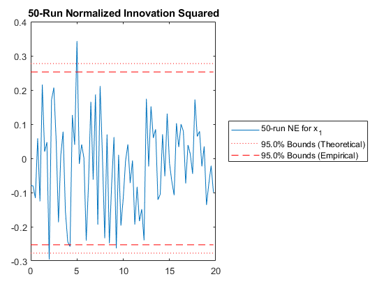
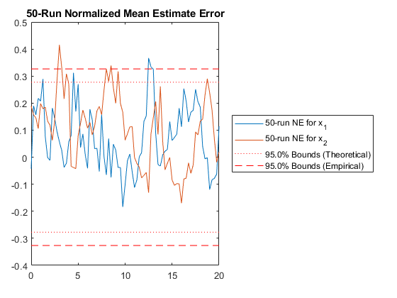
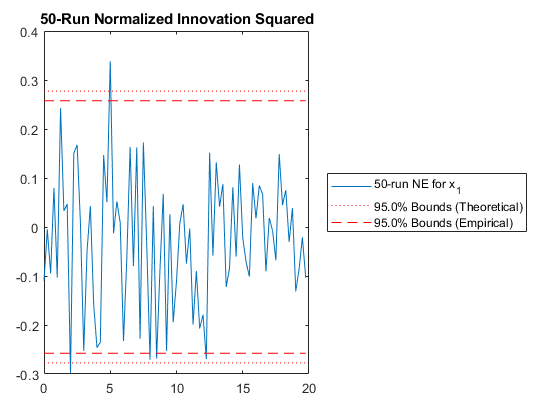
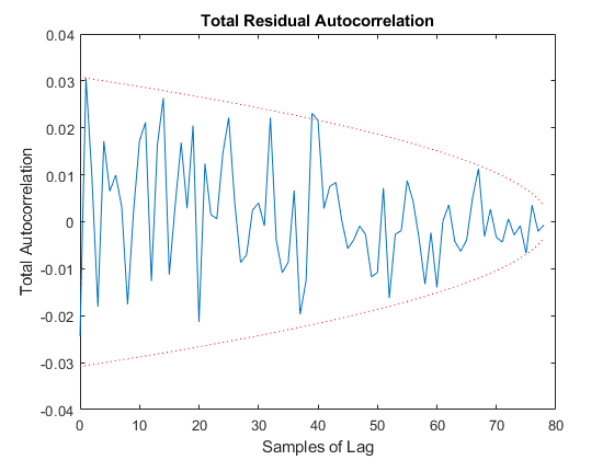
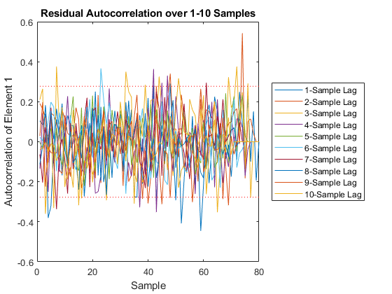
And we can run the Monte-Carlo tests. Because the innovation and its covariance are output, we'll see additional plots and command line outputs telling us how well our filter did. These are similar to the MC's outputs previously, but apply to the innovation instead of the state. The innovation should also be reasonably "white" -- autocorrelation values should be small. Let's see how things go.

jaguar_ekf_mc();

NEES: Percent of data in theoretical 95.0% bounds: 86.4%
NMEE: Percent of data in theoretical 95.0% bounds: 96.3%
NIS: Percent of data in theoretical 95.0% bounds: 97.5%
TAC: Percent of data in theoretical 95.0% bounds: 98.7%
RAC: Percent of data in theoretical 95.0% bounds: 95.3%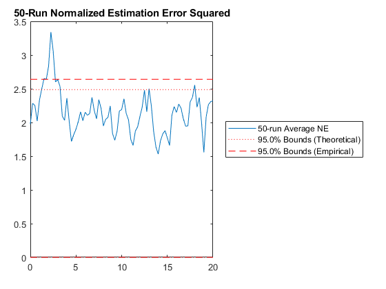

Note that all of the ways of looking at the data show errors reasonably inside the 95% confidence bounds, meaning we likely have a consistent filter that will behave well, within the bounds of our assumptions.

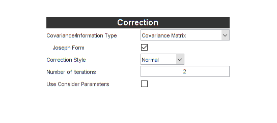
Before we leave Kalman filters behind, let's do one more thing. Kalman filters assume that the measurement noise covariance is known perfectly, but of course ours, which is built from the state estimate itself, certainly has some error. Plus, we necessarily calculate the measurement noise covariance matrix before we update the state (it's used to form the gain that's used to update the state). However, we expect that the updated state is a little more accurate than the prior state. For this reason, it's sometimes effective to use an iterated extended Kalman filter, in which we calculate the measurement noise covariance, update the state, calculate the now-more-accurate measurement noise covariance, and finally re-update the state. This can be done in a loop. Let's use two iterations: the original update, and then one corrected update, to see if it improves our results on the Monte-Carlo test. Set the Number of Iterations to be 2.

Let's regenerate the filter and take a look at the differences:

type jaguar_ekf_step;

 
function [x, P, y_k, P_yy_k] = jaguar_ekf_step(t_km1, t_k, x, P, z_k)
 
% jaguar_ekf_step
% 
% Author: Society of Jaguar Estimators
% Project: Central American Jaguar Studies
% 
% Inputs: 
% 
% t_km1         Time at sample k-1
% t_k           Time at sample k
% x             Estimated state at k-1 (prior)
% P             Estimate covariance at k-1 (prior)
% z_k           Measurement at k
% 
% Outputs: 
% 
% x             Estimated state at sample k
% P             Estimate error covariance at sample k
% y_k           Innovation vector at sample k
% P_yy_k        Innovation covariance matrix at k
% 
% Generated with *kf v1.0.3
 
    %#codegen
 
    % See if we need to propagate.
    if t_k > t_km1
 
        % Create the Jacobian of the propagation function wrt the state.
        F_km1 = population_jacobian(t_km1, t_k, x);
 
        % Create the process noise covariance matrix.
        Q_km1 = population_noise(t_km1, t_k, x);
 
        % Linearly propagate the covariance.
        P_kkm1 = F_km1 * P * F_km1.' + Q_km1;
 
        % Propagate the state.
        x_kkm1 = jaguar_dynamics(t_km1, t_k, x);
 
    % Otherwise, the inputs have already been propagated.
    else
 
        % Explicitly copy the state.
        x_kkm1 = x;
 
        % Explicitly copy the covariance.
        P_kkm1 = P;
 
    end % propagation frame
 
    % Indices of the state that are directly observed
    z_ind = 1;
 
    % Dimension of the state
    nx = length(x);
 
    % Predict the measurement.
    z_hat_k = x_kkm1(z_ind);
 
    % Innovation vector at sample k
    y_k = z_k - z_hat_k;
 
    % State-measurement covariance at k
    P_xy_k = P_kkm1(:, z_ind);
 
    % State estimate used for Jacobians for this iteration
    x = x_kkm1;
 
    % Iterate on the Kalman gain.
    for ii = 1:2
 
        % Create the measurement noise covariance.
        R_k = observation_noise(t_k, x);
 
        % Innovation covariance matrix at k (local)
        P_yy_k = P_kkm1(z_ind, z_ind) + R_k;
 
        % Safely calculate the Kalman gain.
        K = smrdivide(P_xy_k, P_yy_k);
 
        % Update the state estimate.
        x = x_kkm1 + K * y_k;
 
    end % iteration frame
 
    % Build the matrix used for Joseph form covariance correction.
    A = eye(nx);
    A = assign2col(A, -K, z_ind);
 
    % Update the estimate covariance (Joseph form).
    P = A * P_kkm1 * A.';
    P = P + K * R_k * K.';
 
end % jaguar_ekf_step

Finally, let's run the new MC test to see if it's any better than before.

jaguar_ekf_mc();

NEES: Percent of data in theoretical 95.0% bounds: 85.2%
NMEE: Percent of data in theoretical 95.0% bounds: 91.4%
NIS: Percent of data in theoretical 95.0% bounds: 97.5%
TAC: Percent of data in theoretical 95.0% bounds: 98.7%
RAC: Percent of data in theoretical 95.0% bounds: 94.2%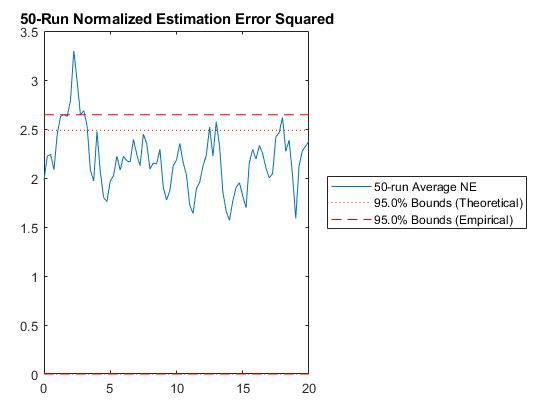

Performance is actually no better. This means that the nonlinearities in our measurement covariance aren't driving the performance. We can leave the iterations on if we like (they don't hurt, statistically), or we can turn them off to speed the filter up a bit.

From here, we could continue to explore options, read the help text that pops up, and generate and examine new filters, but this would go well beyond an introductory tutorial. We've covered UKFs and EKFs, with several options and numerous tests of their quality. Perhaps you're now ready to use *kf with your own problems, and this tutorial should get out of your way. So, before we go, some final tips to help make the most of the *kf engine.

Final Notes and Where to Go Next

We can always save a configuration of the GUI and use it again later by using the Save and Load buttons at the bottom.
The things we set in the GUI can also be set programmatically, without even loading the GUI. See skfoptions and skfgen.
Be sure to check here for a discussion of the shorthand used throughout the documentation.
Though we wrote separate functions for the first and second UKF, we could also use nargin and varargin to determine what the inputs are. This would reduce the amount of code we'd need to write.
We wrote a function for each task, like propagation and observation. Sometimes it's nicer to just use handles to anonymous functions. The *kf frameworks, like kff, allow for this, since they don't generate code.
When working with filters, it's very common to use fixed-step Runge-Kutta methods for propagation. MATLAB does not include fixed-step solvers. While they are easy to program, many solvers, such as rk4, are also available as part of our open-source odehybrid library.

That wraps it up. Thanks for reading!

Problem Statement
Detailed Problem Definition
Building the Unscented Filter
Exercising the Filter
The Generated UKF
Monte-Carlo Testing
Wrap-Up of the First UKF
Another UKF
Linear & Extended Kalman Filters
Jacobians and Noise Covariance
Building the Extended Kalman Filter
Final Notes and Where to Go Next

Docs