by An Uncommon Lab

bf

Run one update of a basic boostrap filter, a type of particle filter, which can estimate well on many types of problems.

 [x_k, X_k, w_k] = bf(t_km1, t_k, X_km1, w_km1, u_km1, z_k, ...
                      f, h, draw_proc_noise, prob_obs_error, ...
                      h_tune);

Inputs

 x_k = fcn([t_km1 t_k], x_km1, u_km1, q_km1)        

 z_k = fcn(t_k, x_k, u_km1)                         

 q_km1 = fcn(t_km1, x_km1)

 p_k = fcn(t_k, dz_k, x_k)                          

 p_k = @(t, dz, x) exp(-0.5 * dz.' * inv(R) * dz)   

 h_tune = (4/(N * (nx + 2)))^(1/(nx + 4));          

Outputs

Example

Let's create an example of localization for a laptop using wifi routers. Suppose we know the locations of several wifi routers across a campus, but we don't know where the laptop is. The laptop can scan and determine the signal strength to each router. It can then run one step of a bootstrap filter. A few moments later, the person carrying the laptop may have moved, but likely not far. Likewise, the signal strength measurements have errors, but we overall know that signal strength diminishes with distance. We should see that we eventually converge on a reasonable estimate of the laptop's position over time.

First, we'll define the true trajectory of the laptop. We'll later use this to produce the measurements of signal strength over time and to determine how well the estimates matched the truth.

% The true trajectory is arbitrary; we'll use a damped velocity random
% walk.
rng(11);             % Set the random number generator for repeatability.
dt = 15;             % Time step
n  = 100;            % Number of steps to take
p  = 30*randn(2,1);  % Random real initial position
v  = [0; 0];         % Real initial velocity is [0,0]
t  = 0:dt:n*dt;      % Time history
x  = [[p; v], zeros(4, n)]; % Full trajectory, with position and velocity
for k = 1:n
    p = p + v * dt;               % Update position
    v = v - 0.2 * v + 0.1 * randn(2, 1); % Update velocity
    x(:,k+1) = [p; v];            % Store the position and velocity
end
 
% Create random wifi router locations over a 200m-by-200m area.
n_routers = 20;
r = 200 * rand(2, n_routers) - 100;
 
% Plot the walk and router locations.
figure(1);
plot(x(1, :), x(2, :), ...
     x(1, 1), x(2, 1), 'ro', ... % Start of walk
     r(1, :), r(2, :), 'r.');    % Router locations
xlabel('East'); ylabel('North'); title('Stroll through Router-Space');
hold on;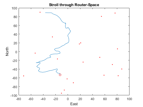

Next, we'll generate the wifi strength to each router at each time step. We'll let wifi signal strength drop as a square of the distance for this example. The measurement vector will be n_routers-by-n_steps.

% Loop over each sample and each router and get the distance from the
% laptop to the router. Also, add noise (10m standard deviation) to the 
% signal strength.
s = zeros(n_routers, n);
for k = 1:n
    for ri = 1:n_routers
        s(ri,k) = 100/norm(r(:,ri) - x(1:2,k+1) + 10 * randn(2,1));
    end
end

Now we need to make propagation and measurement functions that the bootstrap filter will use, but let's suppose we don't know the above (truth) models very well. For instance, let's ignore the velocity and model the propagation as a normal random walk.

% Propagation from sample k-1 to k
f = @(t_km1, t_k, x_km1, u_km1, q_km1) ...
        x_km1 + q_km1; % Just add in the position noise (q_km1)
     
% Measurement for a given sample
h = @(~, x_k, ~) ...
        100./sqrt(sum([r(1,:) - x_k(1); r(2,:) - x_k(2)].^2, 1)).';

We also need two more functions: one to make the propagation noise (the random change in position) and one to determine how unlikely an error in signal strength is. We'll assume the signal strength measurement errors are gaussian, even though in our truth model, they are not.

q_draw = @(~,~) 5 * randn(2, 1); % Draw a random position step
R      = 3^2;                    % Variance of measurement error (!)
r_prob = @(~, dz, ~) exp(-0.5 * sum(dz.^2)/R); % Gaussian error model (!)

Create the initial set of particles as a bunch of random positions and velocities. Also create the weights, which can each just be 1/n_particles since we don't have any idea which particle is best yet.

n_particles = 100;
X = 50 * randn(2, n_particles);
w = repmat(1/n_particles, 1, n_particles);

We've built the entire system and are ready to run the bootstrap filter. For each sample, pass the real signal strength observed for each router into the filter, along with the set of particles and other info. We'll get the updated weighted mean estimate along with the updated set of particles. We can plot the particles as we go.

% Plot initial particle position (all over).
plot(X(1, :), X(2, :), 'g.');
 
% Run the filter for each simulated step.
x_hat = zeros(2, n);
for k = 1:n
    [x_hat(:,k), X, w] = ...
        bf(t(k), dt, X, w, [], s(:,k), f, h, q_draw, r_prob); % Filter.
    plot(X(1,:), X(2,:), '.', 'Color', 0.9*[1 1 1]); % Add particles.
    drawnow(); % Update the plot before looping (animate).
end
 
% Add the estimated trajectory to the figure.
a = plot(x(1,:),     x(2,:),     'b-', ... % Truth
         x_hat(1,:), x_hat(2,:), 'r--');   % Estimate
legend(a, 'Truth', 'Estimate');
hold off;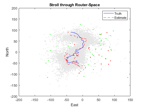

The estimator works very roughly. A more accurate model of the probability of measurement errors would certainly help, as would more particles. A better model of the dynamics (perhaps even the truth model) would require many, many more particles. The ability to use particle filters on problems that are hard to describe is their strength. Their weakness is their extreme slowness and tendency to have particles in unrealistic areas of the state space. However, their are much better forms of particle filter for localization than a basic bootstrap filter. These forms quickly become customized to specific problems.

See Also

ukf