Intro

The odehybrid library for MATLAB makes it easy to create simulations of dynamical systems with both continuous-time components (such as physical models) and multiple discrete-time components (such as digital controllers and signal processors). It's like MATLAB's built-in ode45 function, but extended for discrete-time systems, complex state organization, and logging.

It's open source and free to use even on commercial projects.

We have some quick examples below, and the documentation has a plethora of examples, including all features of odehybrid.

Quick Example

For a stripped-down example, let's simulate an unstable, continuous-time system with a discrete-time stabilizing controller running at 10Hz for 5 seconds.

ode = @(t, x, u) [0 1; 2 0] * x + [0; 1] * u;  % Differential equation
de  = @(t, x, u) deal(x, -[8 4] * x);          % Discrete update equation
dt  = 0.1;                                     % Discrete eq. time step
ts  = [0 5];                                   % From 0 to 5s
x0  = [1; 0];                                  % Initial continuous state
u0  = 0;                                       % Initial discrete state
[t, x, tu, u] = odehybrid(@ode45, ode, de, dt, ts, x0, u0); % Simulate!
plot(t, x, tu, u, 'r.'); xlabel('Time');                    % Plot 'em.
legend('x_1', 'x_2', 'u', 'Location', 'se');                % Label 'em.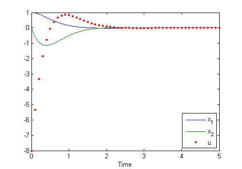

Complex States

Keeping all of the states in a single state vector becomes tedious when managing larger simulations, so odehybrid can take any number of separate states, hand them separately to the continuous-time and discrete-time functions, and return a log of each separately. The states can be matrices, cell arrays, or structs. We'll extend the above example by adding a disturbance to the ODE and an integrator to the controller to handle the disturbance. Note that we can simply add a new input to the ODE, DE, and initial discrete state cell array.

ode = @(t, x, u, i)   [0 1; 2 0] * x ...        % Continuous system
                    + [0; 1] * u ...            %   with feedback control
                    + [0; 1];                   %   and with a disturbance
de  = @(t, x, u, i) deal(x, ...                 % No change to cont. state
                         -[8 4 1] * [x; i], ... % Update input
                         i + 0.5 * x(1));       % Update integrator
dt  = 0.1;                                      % Discrete eq. time step
ts  = [0 5];                                    % From 0 to 5s
x0  = [1; 0];                                   % Initial continuous state
d0  = {0, 0};                                   % Initial discrete states
[t, x, td, u, i] = odehybrid(@ode45, ode, de, dt, ts, x0, d0); % Simulate!
plot(t, x, td, [u, i], '.'); xlabel('Time');                   % Plot 'em.
legend('x_1', 'x_2', 'u', '\int x_1(t)/2 dt', 'Location', 'se'); % Label.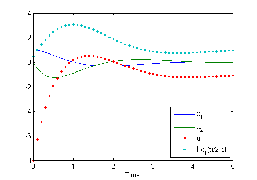

By using separate inputs for separate states and scoping subsystems as fields of hierarchical structs, one can create an elegant system-of-systems simulation.

Logging

Not everything we might want to log is a state, so to log additional values, a logger is included. Just create the log and pass it to odehybrid; it will take care of passing the logger to the ODEs and DEs. It looks something like this:

% Create the logger.
log = TimeSeriesLogger();

% Add inputs for the logger to the ODE and DE.
ode = @(t, x1, x2, ..., log) ... log.add('alpha', t, a) ...;
de  = @(t, x1, x2, ..., log) ... log.add('omega', t, w) ...;

% Provide the logger to odehybrid.
[...] = odehybrid(@ode45, ode, de, dt, ts, x0, d0, [], log);

% Show all of the logged values.
log.plot();

There are many more options for logging. See the documentation for more examples.

Interface

The interface mimics the familiar ode45 interface, expanded for the new material.

[t, ...                      % Output continuous time-steps
 x1, x2, ...,                % Output continuous states
 td, ...                     % Output discrete time-steps
 y1, y2, ...                 % Output discrete states
 te, ...                     % Output event time steps
 x1, x2, ... y1, y2, ...     % Output event states
 ie, ...                     % Output event index
 ] = odehyrbid( ...
        @ode45, ...          % ODE solver
        ode, ...             % ODE
        {de1, de2, ...}, ... % Discrete update(s)
        [dt1, dt2, ...], ... % Discrete update rate(s)
        [0 100], ...         % Time span
        {x1, x2, ...}, ...   % Initial continuous states
        {y1, y2, ...}, ...   % Initial discrete states
        option, ...          % Options from odeset
        log);                % Logger

The ODE function should take all of the states as input and return the time-derivative of each of the continuous states. If a log is provided to , it should also take the log as an input.

[x1d, x2d, ...] = f(t, x1, x2, ..., y1, y2, ..., [log]);

The discrete update functions should take all of the states as input and return the states (including continuous states) as outputs. If a log is provided to , it should also take the log as an input.

[x1, x2, ..., y1, y2, ...] = g(t, x1, x2, ..., y1, y2, ..., [log]);

Installation

1. Download odehybrid from File Exchange.
2. Unzip it to some directory.
3. Add that directory to your MATLAB path.
4. Done! For bonus, check out examples_odehybrid.m.

Contributions

This is an open-source project moderated by An Uncommon Lab. To contribute, please contact us.

Resources

Download it from File Exchange. >>

Blast through the doc. >>

Read about simulations. >>

Read about the motivation. >>

Contact us. >>