How Simulations Work

Intro

People use computer simulations to both understand the world and design for it. Those who need to know where a satellite will be at some future time build simulations of the forces acting on the satellite and propagate its motion from some known location and velocity. Those who design robots create simulations of the environments their robots will experience in order to test how the robots make decisions and move. And those designing power plants simulate weather, energy demand, and system failures to determine the best design for a range of conditions and uncertainty.

However, despite the importance and widespread applicability, few receive education on the subject. The best information is scattered in places one might not know to look, and even most simulation textbooks are narrowly targeted to specific applications or tools. The inevitable result is that many simulations suffer from basic problems that have easy solutions.

This article will set out the critical aspects of building good simulations — that is, simulations that are accurate, easy to develop and analyze, and fast. The first sections deal with how a simulation evolves over time, as this is the core of any simulation. Further sections deal with details that make simulations easier to develop, faster, and applicable to a large number of variations. The target audience is engineers, scientists, and programmers, whether new to creating simulations or experienced. A tiny amount of vector math and calculus is assumed, making this text accessible to first- and second-year undergraduates. By the end, the reader should be able to begin building quality simulations, avoid common pitfalls, communicate the reasons for their decisions to peers, and know where to look for additional resources on specific topics and for the mathematical rigor behind it all.

We'll start with the motivation for understanding the core of how systems evolve over time.

From \(t\) to \(t+\Delta t\)

Let’s get started with a really basic example. Let’s say we have a little moon orbiting a big planet. At some time, we know its position and velocity, and from this we want to simulate the future trajectory.

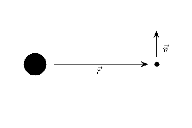
We know the planet pulls on the moon with gravity, so the moon’s acceleration at any point in time is:

$$\vec{a}(t) = -\frac{GM}{r(t)^2} \hat{\vec{r}}(t)$$

Here, \(\vec{a}(t)\) is the acceleration vector, \(\vec{r}(t)\) is the position of the moon with respect to the center of mass of the planet, \(\hat{\vec{r}}\) denotes a unit vector in the direction of \(\vec{r}\), \(r\) denotes the magnitude of \(\vec{r}\), and \(GM\) is the gravitational constant of the planet (remember high school?). Let’s ignore all other forces that might act on the moon for now, since this is overwhelmingly the biggest. How do we turn this into a simulator? It might seem obvious: if we know \(\vec{r}(t)\) and \(\vec{v}(t)\) for some \(t\), then at some time later, \(t + \Delta t\), if \(\vec{v}\) and \(\vec{a}\) are nearly constant across this \(\Delta t\), we would have:

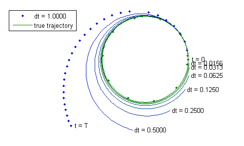
$$\vec{v}(t + \Delta t) \approx \vec{v}(t) + \vec{a}(t) \Delta t$$ $$\vec{r}(t + \Delta t) \approx \vec{r}(t) + \vec{v}(t) \Delta t + \frac{1}{2} \vec{a}(t) \Delta t^2$$

Perhaps by taking a series of small \(\Delta t\) and updating the position and velocity along the way, we'll generate the future trajectory. That certainly seems easy enough, so let's try it out. We'll pick a moon in a circular orbit about the planet. It has a period, \(T\), of 30 time units (we can call them days, but it doesn't really matter) and is located at 1 distance unit from the planet. Since it's a circular orbit, the velocity has magnitude of \(2 \pi / T\) and is perpendicular to the vector from the planet to the moon. Finally, \(GM = \left(\frac{2\pi}{T}\right)^2\). We'll take a series of time steps, each \(\Delta t\) in length. Let's use \(\Delta t\) = 1 time unit, so there should be 30 time steps in the orbit, bringing the moon exactly back to where it started. Here are the results using the “multiply by \(\Delta t\)” method above, plotted on top of the actual future trajectory.

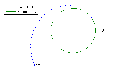
It's not a very good circle. What went wrong?

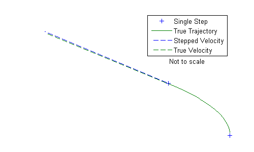
Let's zoom in on the very first time step. Note that as the moon moves, the acceleration should change to always point towards the planet, but since we've assumed the acceleration is constant across \(\Delta t\), the acceleration in this step is always to the left in this figure. This doesn't affect the position all that much, but look at the velocity compared to the true velocity (since this system has a closed form solution, we can compare to an exact value for truth). The stepped velocity wasn't “pulled back” towards the planet enough (since it always pulled left). The result is that the moon is now going a little too fast and to the outside of the true trajectory. This image is not to scale so that we might better see the small difference in the two velocities at the upper left.

As this continues, the velocity will always have a systematic error, leaning to the outside with every step. The error builds up rapidly, and so our simulated trajectory is not useful. Of course, we used a really big time step. Only 30 time steps for the whole trajectory? That seems ambitious. Let's cut the time step down by a factor of 2. And then by another factor of 2. And then again, again, again, and again.

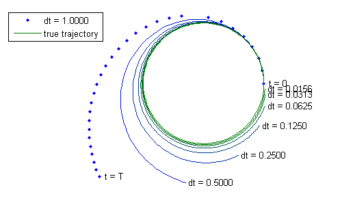
With our smallest time step above we're now taking 1920 time steps, and still the error is huge (given that these are planets).

Now let's fix it. Note that the stepped trajectory is always to the outside, no matter how small the time step. What if we used some method of stepping that wouldn't have this outward tendency? Something that would take a step, see that the new acceleration is significantly different from the acceleration of the previous step, and figure out what the acceleration was across the time step? Fortunately, some great mathematicians have figured out excellent, all-purpose ways to do this. For example, applying one of the most common and all-purpose methods (it's not tailored to orbits in any way), we can achieve less error than our most precise time step above with only 11 steps. Yes, 11. These are plotted as dots on top of the true trajectory below. Let's find out how.

Ordinary Differential Equations

First, we need to establish what types of things we're going to propagate. When we have systems with some state (like position and velocity) at some time and we calculate the derivatives of that state (velocity and acceleration for the example) at that time, we call this an ordinary differential equation (ODE) (and when we're dealing with motion, we call this the equation of motion). We usually stick all of the parts of the state together into a column matrix and call it the state vector.

$$ x(t) = \begin{bmatrix} \vec{r}(t) \\ \vec{v}(t) \end{bmatrix}$$

Then we have this for the time derivative:

$$ \frac{d x(t)}{dt} \equiv \dot{x}(t) = \begin{bmatrix} \vec{v}(t) \\ \vec{a}(t) \end{bmatrix}$$

Then we describe the ODE something like this:

$$ \dot{x}(t) = f(t, x(t))$$ which just states that the derivatives depend on time and the current state and nothing else. It's also common to drop the explicit dependence on time, because it's generally understood. For our example, we have: $$ \dot{x} = f(x) = \begin{bmatrix} \vec{v} \\ -\frac{GM}{r^2} \hat{\vec{r}} \end{bmatrix} $$

When we're keeping track of position by simulating its acceleration, it's a second-order system, because acceleration is the second-derivative of position. However, in terms of the state vector, \(x\), it's a first-order system (we calculate \(\dot{x}\) and not \(\ddot{x}\)). This can cause confusion, so we should just remember that the system is ultimately second-order, and we're just conveniently packaging up everything into \(x\) so as to use first-order techniques on \(x\).

In general, \(f(x)\) is our model of something, which might be nonlinear and even stochastic. The only assumption we make about the whole system is that it's differentiable (smooth-ish). It probably doesn't have a closed-form solution or we'd use the closed-form solution instead of simulating (our circular orbit of course has a closed-form solution, but that's just so that we can compare our simulation to something exact).

We'll talk about other types of systems (things that aren't ODEs) later. For now, this gives us plenty of great material since a plethora of physical systems are described as ODEs that boil down to \(\dot{x} = f(x)\), such as equations of motion, chemical reactions, thermodynamics, population growth, etc. Having a generic framework to describe these systems therefore lets us describe the solvers in a generic way, making them applicable to a great number of different problems.

Fixed-Step Solvers

In the orbit example, we held the acceleration constant across the time step, and this ultimately created a systemic bias to one side. Of course, we could easily have seen that the acceleration wasn't constant across the time step. For instance, we could have propagated by one time step, re-calculated the acceleration, and used this updated value to determine how the acceleration had changed across the time step, allowing us to revise the step. Drawing from this motivation, an excellent solution was created by Carl Runge and Martin Wilhelm Kutta a long while back. They proposed taking a series of small steps forward, using the derivatives along the way to determine the effective derivatives across the entire time step in such a way that the errors could be made very, very small.

Runge-Kutta Fourth Order Method

The most common Runge-Kutta method is known as “the” fourth order method, and we'll call it RK4. It involves calculating the derivatives four times like so:

1. First, calculate the derivative at \(t\), $$ k_1 = f(t, x(t)) $$
2. Form an intermediate update of the state, $$ x(t + \frac{1}{2} \Delta t) \approx x(t) + \frac{1}{2} \Delta t k_1 $$ Use this updated state to calculate another derivative, $$ k_2 = f(t + \frac{1}{2} \Delta t, x(t) + \frac{1}{2} \Delta t k_1) $$
3. Using the new derivative, again approximately update \(x\) from \(t\) to \(t + \frac{1}{2}\Delta t\), and again calculate the derivative. $$ k_3 = f(t + \frac{1}{2} \Delta t, x(t) + \frac{1}{2} \Delta t k_2) $$
4. Finally, use the last derivative to propagate all the way from \(t\) to \(t + \Delta t\), and (you guessed it) calculate those derivatives! $$ k_4 = f(t + \Delta t, x(t) + \Delta t k_3) $$
5. Now we just combine the various \(k_i\) to get the update: $$ x(t + \Delta t) \approx x(t) + \frac{\Delta t}{6}\left(k_1 + 2 k_2 + 2 k_3 + k_4\right) $$

Here it is as pseudocode:

k1 = f(t, x);
k2 = f(t + 0.5 * dt, x + 0.5 * dt * k1);
k3 = f(t + 0.5 * dt, x + 0.5 * dt * k2);
k4 = f(t + dt, x + dt * k3);
xdot = (k1 + 2 * k2 + 2 * k3 + k4) / 6;
x = x + xdot * dt; % x is now updated from t to t + dt.

With this update, the accumulated error is on the order of \(\Delta t^4\), so reducing the time step by a factor of 2 should reduce the error to \(2^{-4} \approx 6\%\) of the original error. This makes it easy to drive the error down to insignificant levels.

Going back to the orbit problem and using this method with a time step of 2.9 days is sufficient to generate the same accuracy as the initial method did with 1920 time steps (and we can start calling that initial method the “Euler” method, though to use his method for a simulation is a bit of abuse of language). Of course, the most expensive part of most simulations is evaluating \(f(x)\), which can be an enormously complex function. For this reason, the number of time steps doesn't actually tell us much about how long our program will take to run to achieve a certain accuracy. Instead, we focus on reducing the number of function evaluations. For the Euler method, we naturally had one function evaluation per time step. RK4 uses four, so instead of comparing 1920 steps to 11 steps, we should more accurately compare 1920 steps to 44. It's still a bargain at about 2.3% of the computational cost for the same accuracy.

This is called a fixed-step solver because \(\Delta t\) doesn't change in response to \(f(x)\), as opposed to adaptive-step methods (below) which do. There are many fixed-step methods of varying degrees of accuracy and purposes. However, RK4 is such a useful combination of accuracy and computational efficiency that, for fixed-step methods, few ever have need to look elsewhere. The author's first aircraft simulation used RK4, and this is still the standard of aircraft simulation texts [Zipfel].

Stability & Accuracy

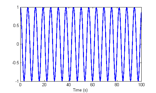
If that's starting to seem too easy, here's where we bring up some concerns. First, we have to pick a time step. It's not always clear how to do that. If the step is too small, the simulation will be slow. If it's too large, important changes in the dynamics might be missed, and weird things can happen — not just wrong or inaccurate, but really weird. For instance, consider the very simple system \(\ddot{x} = -x\). It doesn't get much simpler than that. If we start with \(x = \begin{bmatrix} 1 & 0 \end{bmatrix}^T\), then the system should oscillate forever, making a nice sine wave for all eternity. Here's a simulation using a 0.1s time step.

That looks great, but perhaps we didn't know that 0.1s would be adequate and picked 3s instead. We'd have:

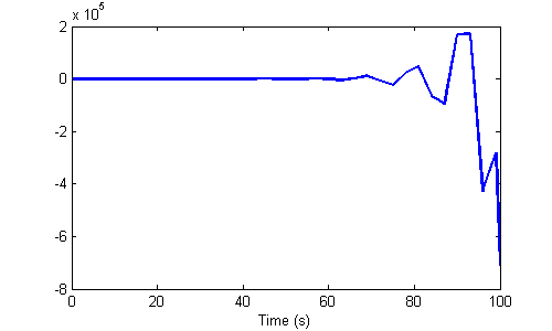
This is not just inaccurate; it's completely unstable. Of course, since our simulation is so simple, it's easy to see that the dynamics are correct, and the solver itself is responsible for the nonsense. However, with much more complicated dynamics, this becomes harder to see. For this reason, one needs to become comfortable starting small and working up to larger time steps.

Further, this points to the bigger message that accuracy and stability are fundamentally different. Accuracy can refer to errors in the models and more-or-less random errors in the results. Inaccurate simulations can still be trusted to a degree (with a nod to the late George Box, we can say that all simulations are wrong, but some are useful). Stability refers to the interaction of the dynamics with the time step and solver algorithm. Unstable results are not just inaccurate; they're complete nonsense. Similarly, we can say that unstable simulations are always wrong and never useful.

For an example of how instability creeps in, let's look at an extremely simplified case: \(\dot{x} = -x\), which as a system is unconditionally stable and should always decay towards 0. It is not possible for this system to ever increase. We'll simulate it with an Euler update (multiply by \(\Delta t\)) from an initial value of 1 with a time step of 3.

\(t\)	\(x\)	\(\dot{x}\)	\(\dot{x} \Delta t\)
0	1	-1	-3
3	-2	2	6
6	4	-4	-12
9	-8	8	24
12	16	-16	-48
15	-32	32	96
18	64	-64	-192

In the system above, we can see that very bad things are happening. On every step, the \(x\) should be 5% of its previous value, and at \(t = 18\), the system should be at 0.000000015. Instead, it's doubling on every step and swapping its sign. This is because the time step is just way too large, using the same derivative for way too long. RK4 has much better stability than the Euler update, but nonetheless it has its limits too.

One could potentially analyze the dynamics to determine an appropriate time step, but in practice, it's easy to just pick a very small time step and increase it to find where a system may become unstable. One can then keep the time step much smaller than this.

Aside from having to pick a time step, another concern when using a fixed-step solver is that one must use a time step sufficient to represent the smallest step that must ever be taken. For things like gentle orbits, this is a good assumption, but for systems that go from rapid changes to slow changes, it means our simulation will be inefficient, as we must use the small time step appropriate for the rapid changes even when the changes are slow. In fact, this brings us to the subject of adaptive-step solvers.

Adaptive-Step Solvers

Let's imagine something like a bouncing ball. While it's in the air, it's a fairly loose system (the acceleration does not change quickly), and a solver could take large time steps. When it's bouncing, the system is very stiff, requiring very small time steps for stability (otherwise, the ball might go through the floor or bounce higher than it started because the forces are so high during the bounce, even for such a short time). To simulate the whole thing with the small step used for the bounce would be wasteful while the ball is moving up and down through the air, where it spends the vast majority of its time. Adaptive-step Runge-Kutta methods provide the means to detect where dynamics are fast and slow, and can therefore automatically pick a time step. For instance, here's a simulation of a bouncing ball using an adaptive-step solver. Note the number of steps (dots) in the air vs. during the bounce.

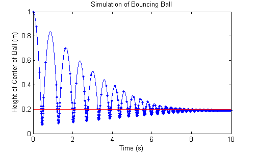
For this simulation, the ball is assumed to be linear-elastic (like a weakly compressed spring). Its dynamics are simple. Let \(x\) be the height of the center of the ball, \(r\) its radius (0.2), \(g\) gravity (-9.81), and \(m\) its mass (1). The ball's acceleration is simply gravity plus any force due to the floor.

$$ \ddot{x} = g + \frac{1}{m} F $$ where \(F\) is the force due to the floor, given by: $$ F = \begin{cases} k (r - x) - b \dot{x} & x < r \\ 0 & x >= r \end{cases} $$

The \(k (r - x) \) term accounts for the force required to compress the ball, and the \(b \dot{x}\) term accounts for energy lost during the impact. For the simulation, \(k\) is 1000 and \(b\) is 2.

The ball is stiff, so the bounce time is very quick. During this short time, the forces on the ball are much, much greater than the force of gravity, and they're changing very quickly as the ball compresses. The adaptive-step solver used for this simulation sees the need to decrease the time step during this period to capture the rapid variation in the dynamics. When the ball is back to the gentle free-fall portion, the solver then sees that it can again increase the time step substantially. The important part is that the solver itself figures this out; we won't explicitly tell it where to make the time step smaller.

Order

To see how this happens, let's first return to our fixed-step solver. The Runge-Kutta method above is described as being fourth order. This means it's accurate to within a fourth-order polynomial approximation of the actual function, centered around \(x(t)\) (that is, the first five terms of a Taylor series expansion about \(x(t)\)), making the local error due to each of these approximations on the order of \(\Delta t^5\). Here's an illustration of three different orders of approximation, each getting more accurate.

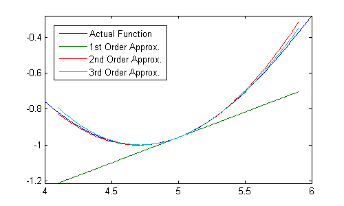
Zooming in, we can still see some error.

The order of a method is determined by the times at which all those derivatives (\(k_1\), \(k_2\), etc.) are taken and the coefficients used to combine them. Simply by taking additional derivatives and recombining how previous derivatives are used, we can create new approximations of the function with different orders. We could then compare the results of one order with those of another order. If a time step is very small, these two approximations will agree very well (as is clear above, where all of the different approximations are very close near \(t = 5\)). As the time step becomes larger, those approximations drift apart. In this way, we can adjust the time step during the propagation to target a certain tolerance for how much they differ (the error). That is, if the error is very small, the time step should increase. If the error is larger than can be tolerated, the time step should be decreased until it's back to within acceptable bounds. This allows the time step to adjust to both fast and slow dynamics automatically.

Algorithm Outline

Unlike RK4, the adaptive-step algorithms are a little long. The good news is that they're not hard to understand, and there are great libraries out there that already implement a variety of adaptive-step solvers, so one would rarely need to program one from scratch. Here's the basic algorithm for a single time step:

While trying to find a valid time step...
  Calculate the set of derivatives, k1, k2, ....
  Form the state update of order x (the higher order).
  Form the state update of order y.
  If the x and y updates are close...
    Update the current state using order x.
    Make the time step larger if need be.
    This time step was valid, so break out of the loop.
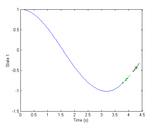
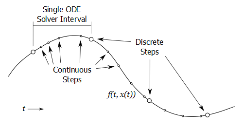
  Otherwise, make the time step smaller and try again.

Let's take a look at an example. Here's a dynamical system where the solver is taking a large time step. The past propagation is shown in blue, the partial state updates are shown as green dots, and their derivatives are shown as line segments extending from the points. The two state updates are shown too, one as a red circle and one as magenta, though in this image, they're right on top of each other.

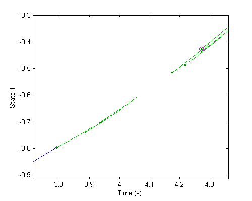
Let's zoom in on the partial state updates. All those green dots are the partial updates of the state, such as the 3 partial updates we made to calculate the derivatives in RK4. The derivatives here are just the slope, shown with a little line segment extending from each point.

Finally, let's zoom way in to see the difference between the two different orders of state update.

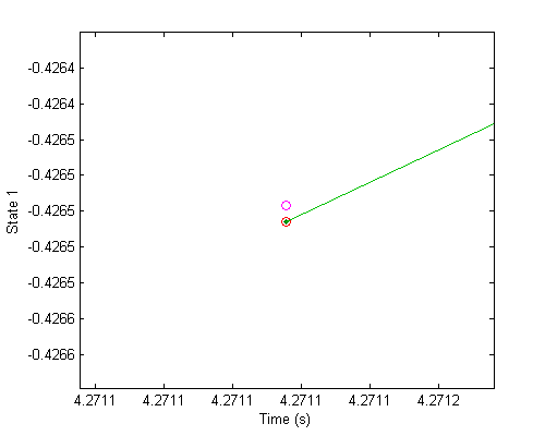
Now we can see the error. Is this too much error or is it ok? That depends on context. There are absolute error tolerances, such as insisting that the error is always less than 1cm. That might make sense for a simulation of planets, but it's a huge error for something like a robotic arm. Then there are relative errors, such as insisting that the error should only be 1% of the magnitude of the state. In practice most implementations of adaptive-step solvers allow for both types of error tolerances. If either is violated, the error is considered too big.

In the example image above, if the error is tolerable, then we use the highest order propagation as our new state, update the time from \(t\) to \(t + \Delta t\), and we're ready for another step. On the other hand, if the error is too big, we throw everything away, reduce the time step, and try again until the two propagations agree well enough.

By taking a series of time steps of different magnitudes and always checking that the error is acceptable after every step, we can propagate from the initial condition until we reach the end time for the simulation.

Efficacy

At this point, it's natural to think that this seems a little wasteful. Whereas RK4 only needs four function evaluations per step, adaptive-step solvers add more function evaluations so that approximations of two different orders can be formed. Further, whenever the step is too large, it must throw out one time step worth of function evaluations in order to try again. Because of this, many people assume adaptive-step solvers are a luxury but not applicable when one needs to make a fast simulation. However, this perception is usually wrong. Most interesting simulations have both fast and slow dynamics at different points (like our bouncing ball simulation), and in this case, adaptive-step solvers can actually execute faster than fixed-step because they can take much larger steps when the dynamics are slow, requiring fewer total steps to finish the simulation and generally fewer function evaluations. Add to that the fact that adaptive-step solvers provide some notion of how much error there is in the simulation and their ability to propagate safely on a large variety of problems, and these in fact can be seen to be excellent tools for simulation.

The are many good adaptive-step methods that follow this general procedure, and there are as many implementations of these methods in various technical programming languages, such as Mathematica, MATLAB, C, C++, Python, and FORTRAN (the mother-tongue of most of these methods; in fact, many other packages still just wrap the old FORTRAN libraries). This means one generally does not need to actually program an adaptive-step solver oneself. In fact, most people that work in simulations have never written an adaptive-step solver. What's important is understanding how they work and what their assumptions and limitations are, which we've discussed a bit above. On the other hand, the author can't in good faith publish this article without at least one good adaptive-step Runge-Kutta method for the curious reader. Therefore, we'll discuss one of the most popular methods called Dormand-Prince fifth order method with embedded fourth order (written as Dormand-Prince 5(4), which we'll call DP54). Readers looking to just get the gist of these methods may wish to skip this section.

Dormand-Prince 5(4)

First, remember all those coefficients we used in RK4, like \(\frac{1}{2}\) and \(\frac{1}{6}\)? We can arrange those in a little table like so:

$$ \begin{array}{c c c c c} 0 & & & & \\ 1/2 & 1/2 & & & \\ 1/2 & 0 & 1/2 & & \\ 1 & 0 & 0 & 1 & \\ & 1/6 & 1/3 & 1/3 & 1/6 \\ \end{array} $$

This is called the Butcher tableau after the guy who first arranged things this way, and it tells us how to calculate each derivative (\(k_1\), \(k_2\), ...) and how to combine those derivatives into the state update. To make it more general, let's write it this way:

$$ \begin{array}{c c c c c c} 0 & & & & & \\ c_2 & a_{2, 1} & & & & \\ c_3 & a_{3, 1} & a_{3, 2} & & & \\ \vdots & & \ddots & & & \\ c_s & a_{s, 1} & & \cdots & a_{s, s-1} & \\ & b_1 & b_2 & \cdots & & b_s \\ & \hat{b}_1 & \hat{b}_2 & \cdots & & \hat{b}_s \\ \end{array} $$

We always calculate \(k_1\) just like in RK4:

$$ k_1 = f(t, x(t)) $$

To calculate \(k_2\), we step \(c_2 \Delta t\) forward in time and we update \(x(t)\) with \(a_{2, 1} k_1\).

$$ k_2 = f(t + c_2 \Delta t, x(t) + a_{2,1} k_1) $$

Unlike RK4, most methods combine multiple \(k_i\) even when calculating derivatives, so for \(k_3\):

$$ k_3 = f(t + c_3 \Delta t, x(t) + a_{3,1} k_1 + a_{3, 2} k_2) $$

So to calculate each \(k_i\), we update time to \(t + c_i \Delta t\) and update the state with \(a_{i,1} k_1 + a_{i, 2} k_2 + \ldots\), like so:

$$ k_i = f(t + c_i \Delta t, x(t) + \Delta t (a_{i,1} k_1 + \ldots a_{i, i-1} k_{i-1})) $$

Note that, since the \(a_{i,j}\) values make a triangle, we can always calculate the next derivative via propagations of the last-calculated derivative. That is, calculating \(k_i\) only depends on the already calculated \(k_1, \ldots k_{i-1}\). We call this explicit calculation of the derivatives.

We do this for all \(s\) derivatives, and we can then calculate the final update as:

$$ x(t + \Delta t) = x(t) + b_1 k_1 + b_2 k_2 + \ldots b_s k_s $$

Recall that adaptive-step methods create two updates of different orders and compare the difference. We've created one update above. The other update looks the same, but uses the \(\hat{b}\) coefficients:

$$ \hat{x}(t + \Delta t) = x(t) + \hat{b}_1 k_1 + \hat{b}_2 k_2 + \ldots \hat{b}_s k_s $$

Now we said that these two updates represent different orders. How do we know what those orders are exactly? It's implied in the table, but not obvious to read. When mathematicians come up with these tables, they do so to target certain properties, like general usefulness, usefulness on specific problem type, etc. They know from the beginning that they want to obtain certain orders, and in doing so derive an elegant table to represent them. So where these tables are documented, there's always a note about what order is meant by the \(b\) row of coefficient and what order is meant for the \(\hat{b}\) row.

(There's no \(\hat{b}\) row in our RK4 table above, because RK4 is a fixed-step method, so it only has a single update instead of the two updates used by adaptive-step methods. Otherwise, the tables are used the same way.)

Now that we know how the algorithm updates and how Butcher tables work, here's the Butcher tableau for the Dormand-Prince 5(4) method:

The \(b\) row represents a fifth-order update, and the \(\hat{b}\) row represents a fourth-order update, hence this is a 5(4) method.

Note that DP54 has an interesting property. The \(b\) coefficients used to update the state (if the error is small enough) are the same as the coefficients for the last row of \(a\). This means the derivative calculated last in a time step will be the same as the derivative calculated first in the next time step. One therefore need not re-calculate it; we can skip the calculation of \(k_1\) and use \(k_7\) from the previous iteration. This is called the first-same-as-last property, and because of this only six function evaluations are necessary — only two more than RK4. Since DP54 provides larger time steps than RK4 (where appropriate), a higher-order update, and error checking, it's obvious why it's so popular.

The next step is to see if the orders agree well enough. We take as the error the biggest difference between any two rows of the two different state updates, \(x\) and \(\hat{x}\). This is the infinity norm, \(\| x - \hat{x} \|_\infty\). If this quantity is smaller than some tolerance, \(\epsilon\), we say the two updates agree, allowing us to accept the time step and move on to the next time step. If this quantity is greater than \(\epsilon\), we decrease the time step and try again.

Instead of calculating the absolute error (above), we might calculate the relative error instead by scaling each element of \(x - \hat{x}\) by the same element of \(x\) or \(\hat{x}\) and then taking the infinity norm.

Whether the time step is accepted or not, the same rule is often used to update the time step for the next step. Since we know the error characteristics of the solver, we can target an error just shy of what's tolerable. Numerous methods exist for this, but a simple method is the following;

$$ \Delta t \leftarrow \sigma \Delta t \left( \frac{\epsilon}{\|x - \hat{x}\|_\infty} \right)^\frac{1}{p+1} $$

where \(p\) is the lower of the two orders (e.g., 4 for DP54) and \(\sigma\) is a safety factor usually between 0.7 and 0.9. This works for both accepted and rejected time steps, increasing or decreasing the step size as necessary.

This concludes the DP54 algorithm. While there is a mess of coefficients to deal with, the method is actually pretty compact given all that it's doing and is very easy to program — a few nested for loops, tables, and function calls. No big deal. Further, once the basic architecture is in place, simply changing out the Butcher tableau allows one to implement an entirely new adaptive-step Runge-Kutta method. For instance, there's a 3(2) method by Bogacki and Shampine that also has great economy and is very broadly used; we can use its coefficients instead of the DP54 coefficients above to implement it [Bogacki-Shampine method].

Other Solvers

The above solvers are an excellent place to start. In very many cases, they're not only easy to use, but sufficiently fast and accurate that few improvements could be made. However, special cases can warrant special solvers. Since this is a general article, we won't go into the specialization in depth, but we'll mention some of the circumstances in which one would seek out a specialized solver.

Model-Specific

One circumstance in which specialized solvers are useful is for certain heavily-studied models. For instance, orbits can be modeled with great accuracy (compared to, say, aircraft, which have more significant unknowns). For this reason, high-order propagations can pay off, and so orbits are often simulated with very high-order methods [Montenbruck and Gill]. When building a simulation, it's always worth checking the industry-specific literature to see if specialized propagators exist either for better stability, accuracy, or efficiency.

Stiff Systems

Aside from industry-specific problems, there are also certain types of problems that have certain solvers. For instance, the stiffness of a problem is hugely important in choosing a good solver. All problems that we've looked at so far are nonstiff, and the solvers are all considered nonstiff solvers. In the case of the bouncing ball simulation a few sections back, imagine that we made the ball stiffer by making \(k\) much bigger. If our original simulation was a lightweight rubber ball, a stiffer system might be a marble falling onto concrete; that system would have much faster dynamics during the bounce. The solver we used would have stability problems and would fail, giving weird results such as the ball going through the floor or bouncing much higher than it started, with the problems getting worse on every bounce.

The key to simulating a stiff system would not be to just use a smaller time step (this would only work to a degree) but rather to use a stiff solver. Whereas we were using explicit Runge-Kutta methods above, stiff solvers constitute implicit methods, where the table of \(a_{i, j}\) values is not lower triangular, but is complete. That is, the \(k_1\) derivative depends on \(k_2\), and vice versa. To resolve these interdependencies, implicit solvers iterate on the calculation of the derivatives until they hone in on a stable set of derivatives and can update the state. This gives them much greater stability, at a significant computational cost. So when should one use a stiff solver? A general guideline is that, if a simulation has rapid oscillations unless the time step is extremely small, it might be called stiff. There is no formal definition or rule, so judgement is necessary. Again, one can start with the (generally more efficient) explicit methods, using small time steps, and if oscillations appear even with tiny steps, one might switch to a stiff solver.

Any textbook on solutions for ODEs will have a section on stiff problems, and many software libraries contain stiff solvers as well [Butcher]. They're generally drop-in replacements for nonstiff solvers, though they take longer to run because they will iterate on the derivative calculations, calling \(f\) many more times than an explicit solver.

Higher-Order Systems

So far, we've simulated several second-order systems (we used the acceleration to update the velocity and the velocity to update the position). However, especially when the second derivative does not depend on the first derivative (our moon simulation's acceleration didn't depend on its velocity), there are specialized solvers. These provide the same accuracy with fewer function evaluations. The most common strategy is called Runge-Kutta-Nyström. Instead of:

$$ \dot{x}(t) = f(t, x(t)) $$

we use:

$$ \ddot{x}(t) = f(t, x(t), \dot{x}(t)) $$

In fact, it's so similar to RK4, that we implement the algorithm for a single time step here [Kreyszig 960], with xd as \(\dot{x}\):

k1 = 0.5 * dt * f(t, x, xd);
K  = 0.5 * dt * (xd + 0.5 * k1);
k2 = 0.5 * dt * f(t + 0.5 * dt, x + K, xd + k1);
k3 = 0.5 * dt * f(t + 0.5 * dt, x + K, xd + k2);
L  = dt * (xd + k3);
k4 = 0.5 * dt * f(t + dt, x + L, xd + 2 * k3);
x  = x + dt * (xd + 1/3 * (k1 + k2 + k3));
xd = xd + 1/3 * (k1 + 2 * k2 + 2 * k3 + k4);

Note that the only difference between k2 and k3 is the updated value for the first derivative. If the second derivative does not depend on the first, then k2 == k3, so we can skip one function evaluation, making this a fourth order update with only three function evaluations. Nice.

RKN4 is certainly not the only strategy for this type of thing. There are improved methods and even adaptive-step methods specifically for second-order systems, and these can improve performance of RK54 by more than 50% (that is, reducing the number of function evaluations by 2). However, the methods are scattered. Advanced textbooks and journals are the place to look for these methods. Rabiei et al. have a nice paper too.

Multi-Step Methods

Up to now, we've covered Runge-Kutta methods because they are so broadly useful. However, there are other types of tools to propagate an ordinary differential equation from some initial condition. A common type is the linear multi-step method. Instead of taking a series of sub-steps of \(\Delta t\), assembling these into a single state update, and then repeating the process for the next step, multi-step methods use a history of derivatives at the state updates. In other words, they use \(f(t, x(t))\), \(f(t - \Delta t, x(t - \Delta t))\), … \(f(t - n \Delta t, x(t - n \Delta t))\) to construct \(x(t + \Delta t)\). Because they don't take and then throw away various small steps, they update with a single function evaluation. This is a primary motivation for multi-step methods.

However, though they can be efficient, they generally have to take smaller steps than RK methods. Further complicating this is the fact that at the start of the simulation, one doesn't have \(f(t - \Delta t, x(t - \Delta t))\), … \(f(t - n \Delta t, x(t - n \Delta t))\) available, and so one must come up with this somehow, such as falling back to RK4. Finally, because they rely on a history, if something changes suddenly (say, something is discretely updated, which we'll cover later), this is not handled well by these methods. Because their gains in efficiency are small (often nonexistent) and they still require another method to get started, multi-step methods often end up being less attractive in implementation. Nonetheless, the Adams-Moulton method is common and relatively efficient where the added complexity is warranted, and Wikipedia has a good discussion of linear multi-step methods, as does [Butcher].

Zero Crossings

Sometimes something needs to happen exactly when a certain condition is reached in the simulation. For instance, an aircraft simulation should probably end when the aircraft's height above the ground goes negative, or maybe we want a time step right when contact occurs between a robotic arm and the thing it's picking up. In situations like this, it's not enough to hope that a time step occurs sufficiently close to the condition; instead, one uses zero-crossing detection to hone in on the time at which the event happens. Some signal over time is used to measure the nearness to the event, and based on the way this signal changes, one can detect very precisely the time at which it crosses zero. For instance, when the plane's at its cruising altitude, it isn't very close to having its height above the ground be negative. However, as the airplane's height is diminishing or the ground is rising up to meet it, the signal (the height) gets smaller.

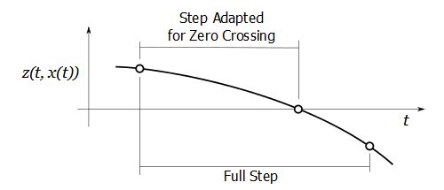
There are simple strategies to determine when the zero-crossing occurs, such as the method of false displacement. Just like for adaptive time steps, when the time step was too large and therefore thrown out, any steps beyond the zero-crossing are thrown out until a step size is chosen that places the signal right at zero. Just like we used \(f(t, x(t))\) for the derivatives, there's usually some function \(z(t, x(t))\) that returns a column matrix of signals. When those signals cross zero, a time step occurs. Any solver could include this behavior after taking a time step to see if it has over-stepped. Though somewhat specialized, some simulation platforms offer this behavior.

Partial Differential Equations

We've looked now at numerous ways to propagate an ordinary differential equation, so one may be wondering what is to be done with partial differential equations. Partial differential equations (PDEs) model not just the evolution of a system over time, but also over other variables, like space. For instance, simulating the state of a fluid over time involves tons of infinitesimal comparisons of fluid in one location with the fluid next to it. PDE simulation techniques are the core behind finite-element methods (such as the mechanical stresses and temperatures throughout a member under load) and computational fluid dynamics (such as the interaction of a wave with a ship at sea).

While there are numerous methods to simulate a system defined by a PDE, they are specialized to particular fields and simulated phenomena, so we could not begin to cover them here. An interesting collection of visualizations of various types of phenomena can be found here.

Discrete and Hybrid Systems

Ordinary differential equations model many types of systems, but certainly not all systems that we care to simulate. For instance, when we simulate a robot, the robot will change from “pick up the bolt” mode to “put it in place” mode as a simple and instant update. We call these instant updates from one state to another discrete, so the robot's software evolves in discrete time, whereas the motion of the robot's arm evolves in continuous time.

Discrete Systems

Discrete updates usually happen on some kind of schedule, and they are very commonly periodic. For instance, let's consider Conway's Game of Life, a simple simulation of subpopulations of some kind of lifeform reproducing and dying over time. The way this works is simple: the lifeforms are spread across a grid, like below.

Here, white cells are empty, and black cells contain a lifeform. At a given moment of the simulation, we calculate how many neighbors a lifeform has (those in adjacent cells of the grid).

• If it's two or three, the lifeform goes on living to the next moment.
• If it's more than three, the lifeform dies due to overpopulation.
• If it's less than two, the lifeform also dies (loneliness? boredom?).
• If a cell has no lifeform, but has three lifeforms in neighboring cells, they reproduce into the empty cell, yielding a new lifeform.

The map of these lifeforms is therefore the state. The function that updates the state is just the little set of rules above, which are applied to the current state. The state is updated, and time proceeds to the next moment, etc. Here's an animation of a random initial state evolving according to the above rules:

The code is quite simple. In the sample below, map is a 2D array of 1s and 0s, with 1 representing a lifeform in the cell. neighbors will be a similar 2D array storing the number of neighbors for each cell. The update step says “update each cell of the map to be 1 (true) where the cell was already populated and has two neighbors or where it has three neighbors; set it to 0 otherwise” (the rules above reduce to this, although it's less intuitive what's going on).

% For each sample...
for k = 1:s

    % Count neighbors using the original map.
    neighbors = count_neighbors(map);

    % Update the map.
    map = (map & neighbors == 2) | neighbors == 3;

end

As might be clear from this simulation, there's quite a bit less math behind the propagation of discrete systems. They're usually just for loops operating on some state for the appropriate number of iterations (samples). To discuss these, let's call the state \(y(t)\) with the associated update function, \(g(t, y(t))\), which operates as \(y(t + \Delta t) = g(t, y(t))\).

When update functions operate at regular intervals (\(\Delta t\) is always the same), we usually work with sample times instead of time. E.g., \(y_{k+1} = g(t_k, y_k)\), where \(y_k\) is the state at the kth sample, \(y_{k+1}\) is the state at the next sample, etc. There's little more to it.

Ensuring Causality

The one subtlety to note is that the changes to the state must be calculated before the state is updated. In the above code snippet, the numbers of neighbors for all cells are calculated before we started changing any of the cells. While it's obvious that one should avoid this in Conway's game, certain programming constructs sometimes obscure it. Object-oriented programming in particular results in a common simulation error of this nature. Consider a fox chasing a rabbit. Here's the update function:

fox.chase(rabbit); % Move fox to intercept rabbit's pos/vel
rabbit.flee(fox);  % Move rabbit directly away from fox
if fox.can_bite(rabbit) % True iff fox is close to rabbit
  disp("Fox wins!");
  stop_sim();
end

With this update strategy, the fox will be properly updated first, but the rabbit can now flee the fox's updated position, which gets time a little backwards (it's acausal). As the fox narrows in on the rabbit, eventually it will step exactly to where the rabbit is running, matching its velocity. However, since the rabbit is updated after the fox, it will for a moment see the fox in front of it and accelerate laterally. The fox can not possibly catch the rabbit, and this result isn't due to the actual dynamics but instead to improper simulation. This code should look something more like this:

% Calculate changes to states.
fox.chase(rabbit); % Record fox's move, but don't update
rabbit.flee(fox);  % Record rabbit's move, but don't update

% Accept state updates in isolation.
fox.update();
rabbit.update();

% Check end conditions.
if fox.can_bite(rabbit) % True iff fox is close to rabbit
  disp("Fox wins!");
  stop_sim();
end

The problem of accidentally-acausal systems is easy to avoid, but only if one makes sure to think about it. Sadly, unwitting programmers make this mistake regularly.

Discrete Event Simulations

Some simulations don't take periodic steps, but instead respond to events. For instance, one might simulate a machine shop as many different machines, each of which takes a certain amount of time to process one job. In this case, it doesn't make sense to step the simulation at a constant \(\Delta t\), but rather to step always to the next event, such as a machine finishing a job or a technician needing a new part. In this case, each machine may have its own update function. The function will output an updated component and the time at which it will be ready. For instance, a milling machine might take a chunk of aluminum as an input and output a milled-out part ten minutes later. The simulation can step a full ten minutes before processing the next step. By combining these types of events into a network, the complex interaction of different systems can provide a picture of likely outcomes. How many parts can we actually complete given the machining limits? How often will an IP packet arrive before the previously-sent packet? Do we have enough waiters on staff tonight?

It's easy to simulate a system in this way; the primary difference from periodic discrete systems is that the time for the next step is an output from the update functions. In the example below, parts are randomly requested. They require work from Machine 1 and then Machine 2, which take different amounts of time. When a machine is given a part to work on, it adds it to its queue. If there's nothing in front of it in the queue, it starts on it right away. Otherwise, it starts the next item when it finishes its current item. When a machine starts an item, it adds a future event (completion of the part) to the list of upcoming events. The simulation steps to each upcoming event and processes it.

while t <= end_time

  % Figure out what happens next.
  [t, event_id] = events.get_next_event_time_and_id();

  % Only run the appropriate event.

  % Generate new random part request on Machine 1; Machine
  % will start if its queue is currently empty.
  if event_id == 0
    machine_1.enqueue(t, Part(), events);

  % Machine 1 finished; give part to M2; start next part;
  % Machine 2 will start if currently empty.
  elseif event_id == 1
    machine_2.enqueue(t, machine_1.get_part(), events);
    end_time = machine_1.start_next_part();
    events.add_event(1, end_time);

  % Machine 2 finishes; store the result; start next part.
  elseif event_id == 2
    finished_parts.add(t, machine_2.get_part());
    end_time = machine_2.start_next_part();
    events.add(2, end_time);

  end

end

fprintf("We finished %d parts.\n", finished_parts.length());
fprintf("There are %d parts in Machine 1's queue.\n", ...
        machine_1.queue_length());
fprintf("There are %d parts in Machine 2's queue.\n", ...
        machine_2.queue_length());

Simultaneous Continuous and Discrete Systems

Things get really interesting when continuous and discrete systems interact. Consider the simulation of an autonomous car. The car's motion is obviously an ODE and should be propagated with an appropriate solver. The car's control system is discrete. It wakes up every \(\Delta t\), reads the most recent information from its sensors, determines what to do, updates itself, and sends the commands to the throttle, steering, and braking systems. It then waits (usually not very long) until it's been \(\Delta t\) from the time it last woke up before doing it all again. We covered ways to simulate both types of systems separately, but how do we combine them?

In fact, there's little to it. We can use a continuous solver from one discrete update to the next and then call the discrete update function at the right time. Afterwards, we can continue propagating with the continuous dynamics, perhaps starting with the second-to-last time step that was used before breaking for the discrete update (the last time step will be cut short so as to end at the right time).

Here's an example system. There's an unstable continuous-time process, a second-order ODE, trying to run off to \(\infty\):

$$ x = \begin{bmatrix} x_1 \\ x_2 \end{bmatrix} $$ $$ \dot{x} = \begin{bmatrix} \dot{x}_1 \\ \dot{x}_2 \end{bmatrix} = \begin{bmatrix} 0 & 1 \\ 2 & 0 \end{bmatrix} x + \begin{bmatrix} 0 \\ 1 \end{bmatrix} u_k$$ where \(u_k\) is the last-updated output of a discrete process. That discrete process, which runs every 0.1s, is: $$ u_k = -\begin{bmatrix} 8 & 4 \end{bmatrix} x - s_{k-1} $$ $$ s_k = s_{k-1} + \frac{1}{2} x_1 $$

Controls engineers will recognize this as a proportional-integral-derivative (PID) controller driving \(x_1\) and \(x_2\) to 0. And here's the simulation's result, with the continuous-time parts shown as smooth lines and the discrete-time parts shown as dots.

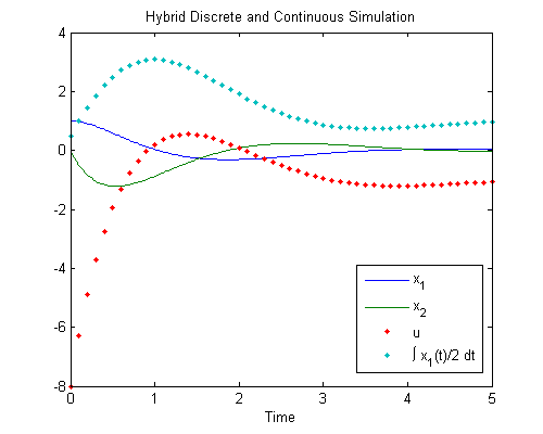
When a continuous state is discretely updated, the continuous states will have two values at a single point in time. For instance, if there's a discrete update at \(t = 3\), then the continuous dynamics will be propagated right up to \(t = 3\), some state update will occur, and then that continuous dynamics will be propagated to the next time step and will start at \(t = 3\). For this reason, we talk about the value of the state at \(t=3^-\), just before the change, and \(t=3^+\), just after it. If one's looking for the value “at” 3s, one must take care to choose the right one for the application.

For instance, let's say a discrete process runs every 0.1s. In this case, the simulator would propagate the continuos states from \(t = 2.9^+\) to \(t = 3^-\). It would run the discrete update, with the updated values corresponding to \(t = 3^+\), and would then continue with the continuous propagation from \(t = 3^+\) to \(t = 3.1^-\).

Extending this hybrid to multiple systems with different periods is direct; we simply have to make sure we break at all of the appropriate times in the right order. We use the continuous-time propagator between those breaks.

When two different systems update at exactly the same time, there's a little ambiguity. Is one supposed to run before the other? Can one use the other's output? This all comes down to what's intended. If a guidance module runs every 10 time steps to update the desired course while an autopilot module runs every time step to keep an aircraft on the desired course, it may be intended that the guidance module run first, followed by the autopilot on those time steps in which both run. On the other hand, if the guidance module is (simulated to be) running in a separate computer from the autopilot, it may be that both run simultaneously, and the autopilot will not see the guidance module's output until the next time step, by which the guidance module has finished its calculation and communicated the values to the autopilot's computer. In the case that two things happen simultaneously, one should buffer the state updates, just like for the corrected fox and rabbit simulation above.

So far, we've covered the very core of most simulations: the evolution of a system over time. Now we'll transition to a series of related topics in no particular order: logging, creating visualizations, extending the simulation into the real world, and incorporating randomness.

Logging and Graphics

Trusting a simulation requires either faith that it was perfectly implemented or good tools for inspection. Most incline to the latter. Since this article is about simulation and not programming practices, we'll just focus on the parts of logging that are relevant specifically to simulations.

Logging

First, discrete-only systems are trivial to log. If one knows a start and end time and the time step, one can preallocate space and fill it with whatever's necessary on each time step. Done.

Continuous-time systems can be more difficult. First, note that our dynamics function, \(f(t, x)\), can't do the logging. Why? Well, recall that with Runge-Kutta methods, it takes several "fake" steps. For fixed-step solvers, these are the intermediate approximations used for the full state update. They should not in themselves be considered state updates, and so they probably shouldn't be logged, at least not the same way as proper state updates. Further, for adaptive-step methods, the entire time step can be thrown out when the step fails! If one had logged at \(f(t + \Delta t, \ldots)\) and then the step was thrown out in favor of a smaller time step, the log would be left with a suspicious value from a fictional and discarded future. For this reason, one generally wouldn't log inside of \(f\). However, the dynamics function is where all of the interesting stuff is happening, so how can one log the interesting stuff? One solution is for the function to take some additional argument that says, “This time, log while you calculate.” The solver could hand in this argument along with the updated state. For instance, it's often useful to log during the calculation of \(k_1\) because this is never thrown away and therefore gives the correct values at the beginning of the time step. (However, it removes the advantage of the first-same-as-last property of the solver, because now \(k_1\) must be calculated at every step.) When using existing libraries, this is often the way to go.

One additional thing to consider while logging is that long simulations can require a lot of memory. If we're using an adaptive-step solver, then we also don't know how many time steps we'll have and must allocate memory somehow as we go. Strategies for dealing with this include: just allocating as necessary and paying the price; over-allocating and filling the buffer, doubling the buffer when necessary; data structures, such as a simple linked list; logging directly to the hard disk.

With these few concerns in mind, logging is generally easy to implement. Otherwise, the only guideline is that it should be easy to add new data to the log. It's mind-numbing to have to edit several files just to see a line plot of a new signal from the simulation.

Graphics

Our brains are organized to process and interpret tremendous amounts of information simultaneously. Simulations of anything other than the most basic phenomena generally require a great deal of interpretation, both after they're finished, and also critically during their development, to understand if the code is working properly. The most common type of visualization is a simple line plot over time, such as we've seen above. These plots of course only show one dimension at a time, and so to understand the interaction between things in the simulation, one must try to mentally synthesize the multi-dimensional picture from these separate plots. That's hard, and we generally miss things when we do this.

Consider that with a good visualization we can display not just three spatial dimensions, but also color, pattern, texture, transparency, connections, annotations, etc. We can see a great deal. Further, when we process things spatially, we have an added boost from our spatial reasoning capability. It's not uncommon for a team to be stunned by discovering something new in their simulation after viewing a 3D animation for the first time, even when they had seen all the information previously as line plots. Simply, we're excellent at processing visual content, and this is an appropriate way to convey the complexity of a simulation in a concise and accurate way.

The good news is that building multi-dimensional visualizations over time isn't actually that hard. Technical computing environments (MATLAB, Mathematica) include tools to draw and manipulate 3D shapes and the ability to animate them over time. Plus, there are many libraries for other languages that can enable fairly easy drawing/rendering. Cinder is a great library for C++. Plus, the Processing language provides an easy way to create visualizations, though it's not recommended for the technical work. As an example of how quickly one can create a visualization with recent tools, consider drawing the planets from our previous moon simulation. The relevant Processing code to animate the 3D planets as simple spheres looks like this:

// Called automatically once to set up scene.
void setup() {
  size(400, 300, P3D);
  background(0, 0, 0);
}

// Called automatically in a loop.
void draw() {

  // ...

  background(0);                                  // Black background
  pushMatrix();
    translate(width/2, height/2, 0);              // Center things.
    float sun = t_now/1000.f * TWO_PI/(12.f*T);   // Move the sun, just for kicks.
    pointLight(255, 255, 255, -1000 * sin(sun), -1000 * cos(sun), 0);
    translate(0, 0, -150);                        // Push the planets deeper into the view.
    noStroke();                                   // Draw planet with no stroke
    fill(64, 196, 64);                            //   with this color
    sphere(50);                                   //   as a sphere with radius 50.
    pushMatrix();
      translate(200.f * x[0], 200.f * x[1], 0.f); // Move to moon's position.
      fill(0, 128, 196);                          // Set moon's color.
      sphere(20);                                 // Draw moon sphere.
    popMatrix();
  popMatrix();
}

It's not a trivial amount of code, but it's easy to get into.

Processing has a bonus: it can be run directly in (most) web browsers. (Safari users, click here.) So here's the planet simulation, running and visualizing directly in the browser (if you see nothing, then your browser isn't compatible):

The complete code for the simulation is available here.

Very often, one runs a complete simulation, logs the relevant data, and then initiates the visualization via the logs. In this way, the visualization can run much faster than the simulation. Similarly, the simulation is not bogged down with visualization (and does not need to be made to run in real-time). Plus, as we covered in the logging discussion, it avoids the problem of trying to draw, only to later have a step thrown out. For drawing while the simulation is running, see the real-time and human-in-the-loop discussion below.

In the Loop

Some simulations are nothing but software. They just run quietly by themselves until they're done. Then one can go look at the results. Other simulations interact with things that aren't just part of the simulation. For instance, a flight simulator might include a joystick for a human to control the simulated aircraft. There are some things to consider about having things in the simulation loop.

Real-Time Simulations

First, there are different meanings for real-time. The easiest is simply that the simulation needs to stay somehow synchronized with an external clock. For instance, suppose it only took 10 minutes to simulate a 3 hour flight. Now, we put a joystick in the system and asked a pilot to fly the plane. Well if the simulation proceeded at 18 times faster than reality, the pilot would be a little challenged to keep up. To be real-time, it generally suffices to have a simulation that runs faster than real-time and to simply insert pauses sufficient to synchronize it with real-time. Alternately, one can attach a function to a periodic callback (a timer), but with this technique, one must be careful about interrupts and threading. If the simulation runs slower than real-time, then one must find a way to change that before one can achieve real-time performance. This is known as soft real-time. Here's a very simple, but reasonably functional single-threaded example.

dt     = 0.1; % Time step
t_last = 0;   % Last time
x_last = ...; % Last state
t_next = dt;  % Next time
while true    % Loop until done
  
  % While waiting for the next update time, draw or otherwise stall.
  while true
  
    % Get the real time.
    t_now = read_a_clock();
    
    % If it's not time to update the state again, just draw or 
    % otherwise fill the passing time with something useful.
    if t_now < t_next
      % Interpolate state from last time to now.
      x_now = interpolate(t_last, x_last, t_next, x_next, t_now);
      draw(t_now, x_now);
    else
      break;
    end
    
  end
  
  % Like as the waves make towards the pebbled shore,
  % So do our minutes hasten to their end;
  % Each changing place with that which goes before,
  % In sequent toil all forwards do contend.
  % ... [Shakespeare, Sonnet 60]
  t_last = t_next;              % What was previously our "next"
  x_last = x_next;              % sample is now our "last", and
  x_next = update(t_next, x_next, dt); % we'll make a
  t_next = t_next + dt;                % new "next".
  
end

Another use of the term real-time implies running the simulation on a deterministic computer (e.g., not OS X or Windows, but something with a real-time operating system) in order to ensure that running a simulation twice will produce exactly the same results and exactly the same times. This is hard real-time and is most useful when designing algorithms that are going to run extremely quickly on regular signals, like communication algorithms and audio processing gear.

In either sense of the phrase, an interesting facet of real-time simulations is that they expose the difference between a simulated world and the simulated computing in that world. For instance, when initially designing a robot's control algorithms and testing them in a simulator, the robot is usually assumed to read its sensors, run a calculation, and output a result to its actuators instantly. However, each of these actions takes time, and it is usually during real-time testing that one finds just how long. Detailed simulations include delays to model these latencies, such as the amount of time it takes a message sent over TCP/IP on some network to actually get to its target (and be interpreted). These are generally buffers of some kind. Here's an example of a buffer storing messages output from a robot's control computer to an actuator far away:

Message	Time Initiated (s)	Time Completed (s)	Time of Arrival (s)
valve21 open	53.100	53.212	53.217
valve22 open	53.100	53.213	53.218
heartbeat	54.450	54.450	54.451

Note that, even once the simulated computer has finished one sample (Time Initiated), we're simulating how long it would have taken the real computer to finish the calculation (hence the Time Completed field). Then, the command still must traverse a network to the target actuator, so the actuator should not be effected until after the Time of Arrival time. This is just a very simple simulation of computational and network latency, but even this can expose serious problems with the underlying control logic, such as unexpected cycles.

Humans in the Loop

Having humans in the loop implies generally some sort of input device (like a joystick, keyboard, buttons, or sensors) as well as outputs for the humans (like a visualization, sound, haptic feedback to controls, etc.). For humans, visualizations tend to work well when they update at 24 frames per second. However, a simulation might have a time step significantly larger than 1/24 seconds. Must one reduce the simulation's time step? In fact no. It's more common to let the simulation run at its appropriate time step and to update the graphics by interpolating from the previous step to the most current. This generally creates smooth performance for the user. However, the performance will be delayed by up to a time step before the user sees it. Humans, fortunately, don't tend to react fast enough for that to matter. Further, any input from the user must be buffered until the simulation steps again, so the inputs are similarly latent. The input-to-output cycle is referred to as latency. Humans can only perceive a latency of 5ms between their actions and the effects, in the most extreme cases. Generally, much higher latency, like 100ms, is quite tolerably “instant” as far as humans can tell (or care).

For this case, the update function called in the example above may look like this:

function x_next = update(t_last, x_last, dt)

  % Read human's input devices (e.g., joystick).
  inputs = read_inputs();
  
  % Update one time step, getting the simulated outputs.
  [outputs, x_next] = step(t_last, x_last, dt, inputs);
  
  % Send any outputs to the human, such as haptic feedback.
  send_outputs(outputs);
  
end

Software in the Loop

Sometimes the purpose of a simulation is to have a simulated environment in which to test an algorithm being designed. For instance, before launching a robot to Mars, one would simulate Mars and test the robot's software inside the simulated environment. Often, one designs algorithms in a high-level language (perhaps the same language as the simulation). One then translates that algorithm to lower-level languages, like C. However, to ensure that one has translated correctly and that the software has the expected behavior, one wraps that software so it can be called from the simulation. This is known as software-in-the-loop testing and is used to ensure that software results agree with the intended design, meet specifications, etc.

Processor in the Loop

Processor-in-the-loop (PITL) testing goes one step further than software-in-the-loop testing. The software is actually put on the target computer. The simulation then provides inputs to the computer from the simulation (such as sensor readings), and it reads its outputs and brings those back into the simulation (such as a “roll forward” command). Processor-in-the-loop testing finds what differences can arise between running a piece of software on a development machine and the actual target environment. For instance, if you were to run a piece of software that used a double on a PC and then ran the exact same code on an Arduino, you would get a different answer, because Arduinos treat the double type as a 32-bit floating point, whereas PCs will treat them as 64-bit. Storing GPS coordinates as 32-bit instead of 64-bit, for instance, can result in meters of error. It's nice to find these problems early.

Depending on the configuration of the target computer and the purpose of the software, PITL tests can be hard real-time, soft real-time, or not real-time at all. For instance, the processor can just wait for a new message from the simulation (a set of inputs for the algorithm), run the algorithm, send back the result, and then wait for the next set of results.

Hardware-in-the-Loop

PITL testing is a type of hardware-in-the-loop (HITL) testing, but hardware can include much more, such as real sensors, emulated sensors, actuators, etc. For instance, to test that the Mars rover responded correctly to illumination conditions, one might have the solar arrays/some illumination sensor running in a room with controlled lighting. The simulation would send out commands to the lights according to the simulated condition, the arrays/sensor would detect the lighting change and send their signals to the central computer (where the software is running). The software would react and send out new commands, which would then be fed back to the simulation, completing the loop. Alternately, the simulation might communicate to devices to pull various digital input/output pins on the target computer high or low, according to what the sensors should be doing, and it might read the output pins and treat those as commands to the simulated actuators

HITL testing is used to find all kinds of conditions and exercise the hardware. It can test how the target computer will ultimately read and write its data while also running a control system, test resource limits that may have been missed, and generally begin to physically affect the world. It can range from rudimentary, which one might implement with a little thought and decent programming skills, to bogglingly detailed, requiring experience, low-level programming, and specialized hardware.

Randomness

This brings us to our final topic: how randomness is included and interpreted in a simulation.

Pseudo-random numbers (henceforth referred to simply as random numbers) are used throughout simulations to model uncertainty and noisy processes, such as wind gusts or thermal noise on an optical sensor. There are a few details one should know when using random numbers in a simulation, and we'll see how these can help one create more accurate and faster simulations with more meaningful results.

Repeatable Random Number Streams

Random number streams are repeatable, meaning they can provide the same set of random numbers multiple times. That is, if one seeds a random number generator (RNG) with x, makes a series of draws from the generator, re-seeds it with x, and makes the same number of draws, both sets of draws will be identical. This is critical in allowing one to re-run a simulation to get exactly the same result, perhaps to further investigate an odd case. It's good practice to store random number generator seeds used at the beginning of a simulation along with the rest of the logged data so that the simulation can be exactly recreated later. Here's an example with MATLAB's random number generator, which can be seeded with rng.

rng(1983);   % Seed it.
randn(1, 5)  % Make 5 draws.
rng(1983);   % Re-seed it.
randn(1, 5)  % Make 5 draws; they're the same!

Output:

ans =
   -0.5420   -0.4530   -0.3680   -0.1231   -2.0084
ans =
   -0.5420   -0.4530   -0.3680   -0.1231   -2.0084

Correlation

A problem that can occur in using multiple random number generators is correlation. When two signals are correlated, one signal follows another signal, but with a delay. In the extreme, if two RNGs are seeded identically, they will produce the same values. This can cause problems. For instance, imagine we're simulating something with a few noisy sensors. We want to add more sensors so that the true signal can be better detected from all the noise, so we add a dozen more sensors. However, if our sensor object has its own random number generator, seeded to 1 by default, then in fact all sensors will read exactly the same value at all times, and adding sensors won't appear to help us eliminate the noise. Similarly bad but less obvious things occur when one random number stream is only a few random draws behind another. Fortunately, seeds don't directly map to “positions” in the random number stream, so seeding one RNG with 1 and the next with 2 will result in two effectively uncorrelated random number streams for most libraries.

Randomness in ODEs

A particularly insidious problem in many simulations also often goes unnoticed. It happens when one uses a random number generator within the differential function used by an adaptive-step solver. Remember how those solvers maintain solutions of two different orders, measuring how much they disagree? If there are separate random draws in the different calls to \(f(t, x(t))\), then the results will differ, making the solver believe that a smaller time step is required. This causes the simulation to take extremely small steps, making the simulation take substantially longer. However, this problem can always be avoided.

If a random number is really just used by a discrete function (such as a sensor reading), the random draw should be taken directly in the discrete function and not the continuous function. This is the easy case.

The harder case occurs when the random number is used in the continuous-time dynamics. However, that does not mean the random draw must actually be taken inside of \(f\). Consider DP54. There are two samples calculated at \(t + \Delta t\) (see the two 1s on the left hand side of the Butcher tableau). However, it makes no sense to return two different derivatives there due to two different draws. Bear in mind that the whole time step represents the physical process, with the sub-steps meant to get the derivatives right. Therefore, if we can reduce the effect of the random number stream on the derivatives to something smooth across the step, we will have effectively represented the random number stream in the dynamics, while allowing a physically meaningful (and larger) time step.

One method is to use a discrete update to add the “noise” from the random draw. For instance, let the modeled acceleration (\(\dot{v}\)) of something be affected by some kind of white noise with mean \(\mu\) and variance \(\sigma^2\).

Clearly, the velocity would be updated something like:

$$ v(t + \Delta t) = v(t) + \int_t^{t+\Delta t} \dot{v}(\tau) d\tau $$

But this integral doesn't really work for us. Imagine using a continuous-time solver; the derivatives would always be different, so the time step would be reduced until \(\Delta t \sigma\) was lower than the error tolerance. The good (great!) news is that this is something called a Wiener process after the mathematician who proved that it reduces to the following much simpler expression:

$$ v(t + \Delta t) = v(t) + \Delta t \nu $$

where \(\nu\) is a Gaussian random variable related to the previous mean and variance as:

$$ \nu \sim \mathcal{N}(\mu, \frac{\sigma^2}{\Delta t}) $$

That is, it's a Gaussian random number with the same mean and scaled variance, and it's held constant across \(\Delta t\). Because of this, we don't need a bunch of little random draws; one will do it!

In general, if our ODE looks like this:

$$ f(t, x) = \ldots + \omega $$

where \(\omega\) is white noise with mean \(\mu\) and variance \(\sigma^2\), then we can replace the noise with:

$$ f(t, x, \nu) = \ldots + \nu $$

where \(\nu\) is drawn at the beginning of each sample using the distribution:

$$ \nu \sim \mathcal{N}(\mu, \frac{\sigma^2}{\Delta t}) $$

This will create an addition of \(\Delta t \nu\) across the time step. Note that this assumes that the noise is relatively small compared to the process represented by \(f\). The approximation holds best when \(\Delta t\) is small, but since we're modeling the effect of noise to begin with, one needn't get too carried away worrying about the approximation.

To create this random draw as code would look something like this:

nu = mu + 1/sqrt(dt) * sigma * randn();

where randn() produces a discrete random draw from a Gaussian distribution with zero mean and unit variance. The solver would then need to do something like this (using RK4 as an example):

nu = mu + 1/sqrt(dt) * sigma * randn();
k1 = f(t, x, nu);
k2 = f(t + 0.5 * dt, x + 0.5 * dt * k1, nu);
...

While the discussion of what's necessary took some time (and probability theory), in fact the implementation, as above, is very simple, and with this, we can create stochastic effects in simulation that are both more accurate and substantially faster than putting the random draw directly inside of \(f\).

Monte Carlo Simulation

By simply running the simulation a bunch of times with different random number seeds or choosing different initial conditions in some sufficiently random way, we can gain insight into the robustness of certain phenomena in the simulation (the ability of the robot to catch the ball, the probability that a storm will hit New York, the utility of some investment, etc.). Believe it or not, this simple strategy of running a bunch of simulations has a name: Monte Carlo simulation, referring to the randomness of dice rolls and card shuffles in the famous gambling haven. The pseudocode usually looks something like this:

n = 10000;                       % We'll run 10,000 simulations.
results = {1, 10000};            % Make some space for the results.
for k = 1:n                      % For each simulation...
  rng(k);                        %   Set random number generator seed.
  x0 = draw_initial_condition(); %   Initialize with draws.
  xf = simulate(x0);             %   Run simulation, also with draws.
  results{k} = xf;               %   Store the result.
end
analyze(results);                % Do something with the results.

There is a subtlety here though. Say we ran 100 simulations, and some event happened in 15 of them. Do we conclude that the event happens 15% of the time? Maybe. Of course, it all depends on what those 100 simulations ultimately meant. To give an example, suppose we're simulating a player throwing a basketball from the free-throw line. We've added random draws to account for the variation in velocity of the ball leaving the player's hands, the air density that day, the movement of the air (inside/outside), etc. Since we're simulating one type of thing with properly distributed random number draws, then yes, we should conclude that the player makes the basket 15% of the time.

Now let's consider a different example: simulating a coworker throwing a crumpled piece of paper across his cube into a recycling bin. He makes it with alarming frequency, but misses with weird weights of paper and the occasional lop-sided crumple. Let's say the probability of a weird weight is 2% and the probability of a lop-sided crumple is 5%. Instead of simulating 1000 cases to determine how frequently he makes it in general, we could simulate 50 cases of normal paper, normal crumple, 50 cases of weirdly-weighted paper/normal crumple, 50 cases of normal paper/weird crumple, and 50 cases of weird/weird. Here are the results:

Weight	Crumple	Baskets
Normal	Normal	48/50
Weird	Normal	37/50
Normal	Weird	23/50
Weird	Weird	19/50

While that's 200 simulations total, of which 127 went in the basket, we can't conclude that the probability of making the basket is 126/200 * 100% = 63.5% because the simulations aren't all equally likely. We know that the weird/normal and normal/weird conditions happen less often than normal/normal, and weird/weird almost never happens. Instead, we'd weight the results. In our example, the probability of normal weight and normal crumple is (1-0.02) * (1-0.05) = 0.931, weird/normal is 0.02 * (1-0.05) = 0.019, normal/weird is (1-0.02) * 0.05 = 0.049, and weird/weird is 0.02 * 0.05 = 1e-3. Thus, the general probability of the coworker making a basket is:

  (1-0.02) * (1-0.05) * 48/40 ...
+ 0.02     * (1-0.05) * 37/50 ...
+ (1-0.02) * 0.95     * 23/50 ...
+ 0.02     * 0.95     * 19/50

which comes to 93% — very different from the 63.5% we erroneously calculated earlier.

If instead, we had run 10,000 simulations, letting 2% of the runs have weird weight and 5% of the runs have weird crumples, and then summed up the number of baskets, we'd find something like 92%.

The lesson here is two-fold. First, one must make sure to account for the probabilities of the events one is simulating. Second, one can break simulations apart to focus on areas with distinctly different probability, and nonetheless reconstruct a picture of the entire simulation with relatively few simulations.

Formalizing this process of running a small number of simulations (tests) to determine overall performance with careful sampling is part of a field known as design of experiments. A good statistics book will have material on this.

Chaos and Complexity

Simulation of a dynamics function is fun. The interaction of even simple models can create tremendous complexity, the interpretation of which will take far longer than the construction of the simulator. Of course, with so much complexity comes an element of chaos. Long ago, early dynamicists noticed that some of the very first simulations built on computers were doing something odd. Even without random number draws, running the simulation twice with the same inputs resulted in dramatically different behavior. When they examined the situation further, they found that in fact the inputs were very, very slightly different, at the level of computer round-off. And yet, the simulation wasn't wrong. In fact, small differences affected the initial small patterns that formed, which affected later patterns, etc., until the final results appeared to show different things. If one changes a gain in an aircraft simulation from 8 to 8.000000001 and suddenly the plane doesn't fly, that's a problem. But if one changes the initial state of a weather simulation ever so slightly, and a storm emerges in the updated simulation, this may actually be correct (this is one reason weather patterns are so difficult to predict). Certain simulations are much more likely to exhibit this than others. Simulations of feedback control systems, like an autonomous sail boat, should be pretty consistent (the boat will arrive in Honolulu at about the same time when initial conditions are changed slightly). Simulation of uncontrolled systems with large numbers of interacting agents, however, can exhibit this behavior. If a system is thusly complex, running Monte-Carlo simulations of different initial conditions can be used to understand the likelihood of the various outcomes (e.g., in 90% of the simulations, New York was just windy, but in 10% of the simulations, it rained). Dr. Melanie Mitchell has an excellent introductory book on the subject called Complexity.

Summary

We've looked at ways to make simulations that are correct, easy to work with, and fast, and we've covered enough material to enable one to build effective simulations for one's own models, whatever industry those might be in. From here, one can pick and choose which aspects require more depth and fidelity. In order to help with this, the author would love to suggest a single good book on simulation itself. Alas, he has been unable to find such a book. However, since there are many great textbooks on various subjects that all have sections crucial to building good simulations, a summary of these books will serve as a summary of the content we have covered herein and where to look next, so this is how we will conclude.

• If simulating ODEs in any form, a solid reference is necessary on the numerical techniques of solving the initial value problem.
• When a discrete system is in fact a control system, a controls textbook should suffice to discuss discretization and state transitions.
• A systems theory book is useful in understanding what results might be expected from various constructs and especially for understanding stability.
• An industry-specific textbook on modeling practices often covers the basics of several of these subjects to an introductory degree. In rare cases, such textbooks can provide the lion's share of information necessary to build a useful simulation.
• Most graphics systems have many little facets, so a good graphics reference is helpful, such as the OpenGL Superbible, Cinder API, the manual for a software package, etc.
• A statistics book will be a good reference when adding stochastic content to a simulation and will be further useful in intelligently interpreting the results. When one begins to view a simulation as an experiment, then the design of experiments becomes particularly useful, and any good statistics book should cover this.
• Finally, though we didn't cover it here, simulation is only the beginning, after which analysis takes over to make real meaning of the results of the simulation. Sometimes increasing the fidelity of a simulation does not do as much to further one's understanding of a phenomenon as would good analysis.

The author hopes this resource has been helpful. Happy simulating!

Resources

Here are a few cited or otherwise useful and interesting resources. Some resources are available online, so these are linked. Otherwise, links to Google Books are provided for the books. If you have access to a technical library, such as a company's or university's, that is likely the best of all.

Articles

Numerical Solution of Second-Order Ordinary Differential Equations by Improved Runge-Kutta Nystrom [sic] Method by Faranak Rabiei, Fudziah Ismail, S. Norazak, and Saeid Emadi. A useful paper on improved, fixed-step Runge-Kutta Nyström methods.

Bogacki-Shampine method. A simple discussion of the Bogacki-Shampine method and Butcher tableau on Wikipedia.

Linear multi-step methods. A detailed discussion of linear multi-step ODE propagation on Wikipedia.

Books

Numerical Methods for Ordinary Differential Equations by J. C. Butcher. For deep information on propagating ordinary differential equations, including nonstiff, stiff, one-step, and multi-step solvers. This is where to look for mathematical formalism.

Numerical Methods for Ordinary Differential Equations: Initial Value Problems by David F. Griffiths and Desmond J. Higham. Yes, this has the same title as the Butcher book. This is an introductory text with many examples and algorithms for the basics of ODE propagation. The breadth of this book makes it useful in practice.

Advanced Engineering Mathematics by Erwin Kreyszig. Such a broadly useful book that perhaps all technical bookshelves should contain a copy. Covers a wealth of subjects, including three excellent chapters on numerical methods. Chapters 17 and 19 are particularly useful in relation to simulation. Check out the used prints of ninth or eighth editions.

Satellite Orbits: Models, Methods, and Applications by Montenbruck and Gill. This is quite possibly the best single book on simulation of spacecraft and includes a short but apt discussion of solvers.

Modeling and Simulation of Aerospace Vehicle Dynamics by Peter Zipfel. Excellent book for aircraft simulation for a huge variety of reasons. Relies on RK4 for the ODEs.

Software

odehybrid is a set of open-source simulation tools for MATLAB, including fixed- and adaptive-step propagators, a hybrid continuous- and discrete-time engine, methods to organize complex states into the forms needed for simulation, and a logging tool.

Simulink® is a simulation environment from The MathWorks for hybrid system simulation, design, verification, and code generation.

Cinder is a visualization library for C++ focused on making many types of visualization much easier than more traditional approaches.